Updated: February, 2017
 Over the years I’ve spent a fair amount of time thinking about radiometric dating techniques as compared to other means of estimating elapsed time. But why is this topic so interesting and important for me? Well, for many former and even current Seventh-day Adventists, radiometric dating of the rocks of the Earth presents a serious problem when compared to the apparent claims of the Bible regarding a literal 7-day creation week – and many have voiced such concerns over the years (Link). After all, according to nearly all of the best and brightest scientists on the planet today, life has existed and evolved over many hundreds of millions of years.
But how can they be so sure? Their confidence is primarily based on the fact that radioactive elements decay or change into other elements at a constant and predictable clock-like rate. And, these radiometric “clocks” certainly appear to show that living things have in fact existed and changed dramatically on this planet over very very long periods of time indeed!
So, why is this a problem for so many within the church? Well, the Seventh-day Adventist Church, in particular, takes the Bible and the claims of its authors quite seriously. Of course, this creates a problem…
Table of Contents
- 1 What did the Authors of the Bible Intend?
- 2 The Basic Concept Behind Radiometric Dating:
- 3 The Potassium-Argon Dating Method:
- 4 The Argon-Argon Method:
- 5 The Uranium-Lead Dating Method:
- 6 Cosmogenic Isotope Dating:
- 7 Fission Track Dating:
- 8 Carbon 14 Dating:
- 9 Assuming A Literal Creation Week and a Noachian-Style Flood:
- 9.1 Before the Flood:
- 9.2 Lord Kelvin and the Age of the Earth:
- 9.3 Increased Radioactive Elements on the Surface of the Planet:
- 9.4 Where did All the Water Come From? and Go?
- 9.5 Bioturbation:
- 9.6 Warm world:
- 9.7 World-wide Paleocurrents:
- 9.8 Lack of Ocean Sediment:
- 9.9 Lack of Erosion:
- 9.10 DNA Mutation Rates as a Clock:
- 9.11 DNA Decay – Devolution not Evolution:
- 9.11.1 Overall mutation rate:
- 9.11.2 Functional DNA in the Genome:
- 9.11.3 Implied functional mutation rate:
- 9.11.4 Ratio of beneficial vs. detrimental mutations:
- 9.11.5 Detrimental mutation rate:
- 9.11.6 Required reproductive/death rate to compensate for detrimental mutation rate:
- 9.11.7 But what about the effect of beneficial mutations?
- 9.12 Rapid Speciation:
- 9.13 Circaseptan (7-day) circadian rhythms:
- 9.14 Related
What did the Authors of the Bible Intend?
 The authors of the Bible are quite consistent in their claims that life did not evolve from simple to complex over vast eons of time via a very bloody and painful process of survival of the fittest. Rather, these authors claim that God showed them that all the basic “kinds” of living things on this planet were produced within just seven literal days and that there was no death for any sentient creature until the Fall of mankind in Eden. It is also quite clear that these authors were actually trying to convey a literal historical narrative – not an allegory. They actually believed that what they wrote was literal history. Take, for example, the comments of well-known Oxford Hebrew scholar James Barr:
Probably, so far as I know, there is no professor of Hebrew or Old Testament at any world-class university who does not believe that the writer(s) of Genesis 1–11 intended to convey to their readers the ideas that: (a) creation took place in a series of six days which were the same as the days of 24 hours we now experience. (b) the figures contained in the Genesis genealogies provided by simple addition a chronology from the beginning of the world up to later stages in the biblical story (c) Noah’s flood was understood to be world-wide and extinguish all human and animal life except for those in the ark. Or, to put it negatively, the apologetic arguments which suppose the “days” of creation to be long eras of time, the figures of years not to be chronological, and the flood to be a merely local Mesopotamian flood, are not taken seriously by any such professors, as far as I know.
Letter from Professor James Barr to David C.C. Watson of the UK, dated 23 April 1984.

For many, this sets up quite a conundrum. What to believe? – the very strong consensus of the most brilliant minds in the world today pointing to what seems to be overwhelming empirical evidence? – or the “Word of God” in the form of the claims of the human writers of the Bible? How does one decide between these two options? For me, I ask myself, “Where is the weight of evidence” that I can actually understand for myself?
Now, I can only speak for myself here, but for me the weight of evidence and credibility remains firmly on the side of the Bible. One of the many reasons that I’ve come to this conclusion is that I’ve studied the claims of many Biblical critics for most of my adult life, to include the very popular claims of the modern neo-Darwinian scientists, and I’ve found them to be either very weak or downright untenable – and this includes the popular claims regarding radiometric dating methods in general, which will be the focus of this particular discussion.
The Basic Concept Behind Radiometric Dating:

All radiometric dating methods are based on one basic concept. That is, radioactive elements decay at a constant rate into other elements – like a very steady and reliable clock. Of course, it is now known that this rate is somewhat variable and can be affected by solar flares and other factors (Link). However, from what is known so far, the degree of variation caused by these factors appears to be fairly minimal. So, the ticking of the clock itself still remains fairly predictable and therefore useful as a clock. Of course, in order to know how long a clock has been ticking, one has to know when it started ticking. Also, even if the actual ticking of the clock is reliable, one has to know if any outside influence has been able to move the hands of the clock beyond what the mechanism of the clock itself can achieve. Of course, this is where things get a little bit tricky…
The Potassium-Argon Dating Method:
The only “Pure” Method:
 Why do I start with the potassium-argon (K-Ar) dating method? Well, for one thing, it is the only radiometric dating method where the “parent”, or starting radioactive “isotope” or element in a volcanic rock or crystal, can be pure – without any “daughter” or product isotope already present within the rock or crystal that one is trying to date.
“The K-Ar method is the only decay scheme that can be used with little or no concern for the initial presence of the daughter isotope. This is because 40Ar is an inert gas that does not combine chemically with any other element and so escapes easily from rocks when they are heated. Thus, while a rock is molten, the 40Ar formed by the decay of 40K escapes from the liquid.”
The Most Common Method:
 Because of this feature where only the parent product starts off in a solidifying rock, and because of its relative abundance within the rocks of the Earth, the K-Ar dating method is by far the most popular in use today. Around 85% of the time, the K-Ar method of dating is used to date various basaltic rocks from around the world.
 radioactive 40K decays into 40Ar, the 40Ar gas becomes trapped in the solid crystals within the lava rock – and can’t escape until they are reheated to the point where the 40Ar gas can again escape into the atmosphere. So, all one has to do to determine the age of a volcanic rock is heat up the crystals within the rock and then measure the amount of 40Ar gas that is released compared to the amount of 40K that remains. The ratio of the parent to the daughter elements is then used to calculate the age of the rock based on the known half-life decay rate of 40K into 40Ar – which is around 1.25 billion years. Actually, 40K decays into two different daughter products – 40Ca and 40Ar.
 However, since the original concentration of calcium (40Ca) cannot be reasonably determined, the ratio of 40K vs. 40Ca is not used to calculate the age of the rock. In any case, the logic for calculating elapsed time here appears to be both simple and straightforward (see formula for the calculation). Basically, when half of the 40K is used up, 625 million years have passed – simple!
When Some Argon gets Trapped:
 What happens, though if all the 40Ar gas does not escape before the lava solidifies and the crystals within it have already started to form? Well, of course, some of the 40Ar gets trapped. This is called “extraneous argon” in literature. Experimental studies done on numerous modern volcanoes with historically known eruption times have been evaluated. And, about a third of the igneous rocks from these volcanoes show a bit of extra 40Ar – usually enough extra 40Ar to make the clock look older by a few hundred thousand to, rarely, up to a couple million years. Overall, however, such errors are relatively minor compared to the ages of rocks usually evaluated by K-Ar dating (on the order of tens to hundreds of millions of years). So, although often cited by creationists as somehow devastating to the credibility of K-Ar dating, this particular potential for error in the clock actually seems rather minor – relatively speaking (see illustration). It certainly doesn’t seem to significantly affect the credibility of rocks dated by the K-Ar method to tens or hundreds of millions of years – at least not as far as I have been able to tell. So, where’s the real problem?
Function of Pressure and Rates of Cooling:
Under Water:
 As it turns out, the amount of excess 40Ar is a direct function of both the hydrostatic pressure and the rate of cooling of the lava rocks when they form – under water (Dalrymple and Moore, 1968). This means that, “many submarine basalts are not suitable for potassium-argon dating” (Link). This same rather significant problem is also true for helium-based dating (decay of uranium and thorium produces 4He). For example, “The radiogenic argon and helium contents of three basalts erupted into the deep ocean from an active volcano (Kilauea) have been measured. Ages calculated from these measurements increase with sample depth up to 22 million years for lavas deduced to be recent. Caution is urged in applying dates from deep-ocean basalts in studies on ocean-floor spreading” (Link).
Within Pre-formed Rock:
The “True Age” When K-Ar Dating Goes Wrong:
 So, what is the “true” age of these rocks? If the K-Ar levels cannot be trusted, what other clock is more reliable? In this line consider that the Himalayan mountains are thought, by most modern scientists, to have started their uplift or orogeny some 50 million years ago. However, in 2008 Yang Wang et. al. of Florida State University found thick layers of ancient lake sediment filled with plant, fish and animal fossils typically associated with far lower elevations and warmer, wetter climates. Paleo-magnetic studies determined that these features could be no more than 2 or 3 million years old, not tens of millions of years old. Now that’s a rather significant difference. In an interview with Science Daily in 2008, Wang argued:
“Major tectonic changes on the Tibetan Plateau may have caused it to attain its towering present-day elevations, rendering it inhospitable to the plants and animals that once thrived there as recently as 2-3 million years ago, not millions of years earlier than that, as geologists have generally believed. The new evidence calls into question the validity of methods commonly used by scientists to reconstruct the past elevations of the region. So far, my research colleagues and I have only worked in two basins in Tibet, representing a very small fraction of the Plateau, but it is very exciting that our work to-date has yielded surprising results that are inconsistent with the popular view of Tibetan uplift.” ( Link )
Now, I’m sure that if the organic remains in this region were subjected to carbon-14 dating, that ages less than 50,000 years would be produced. After all, given the significant discrepancy suggested already, I’m not sure why Wang didn’t go ahead and try to carbon date these lake sediments? In any case, this finding of 2-3 Ma for lack sediments still contrasts sharply with mainstream thinking that these regions should be around 50 million years old.
Too Old or Too Young:
What this means, then, is that different methods of measuring elapsed time over very long periods of time often yield very very different results. Sometimes, the K-Ar ages is far to old. And, sometimes, the K-Ar age is far too young. For example, isotopic studies of the Cardenas Basalt and associated Proterozoic diabase sills and dikes have produced a geologic mystery. Using the conventional assumptions of radioisotope dating, the Rb-Sr and K-Ar systems should give the same “ages”. However, it has been known for decades now that these two different methods actually give very different or “discordant” ages with the K-Ar “age” being significantly younger than the Rb-Sr “age”. Various explanations, such as argon leakage or that a metamorphic event could have expelled significant argon from these rocks haven’t panned out (Link). The reason for this, as cited by the New Mexico Research Lab, is that the basic assumptions behind K-Ar dating cannot be known with confidence over long periods of time:
Because the K/Ar dating technique relies on the determining the absolute abundances of both 40Ar and potassium, there is not a reliable way to determine if the assumptions are valid. Argon loss and excess argon are two common problems that may cause erroneous ages to be determined. Argon loss occurs when radiogenic 40Ar (40Ar*) produced within a rock/mineral escapes sometime after its formation. Alteration and high temperature can damage a rock/mineral lattice sufficiently to allow40Ar* to be released. This can cause the calculated K/Ar age to be younger than the “true” age of the dated material. Conversely, excess argon (40ArE) can cause the calculated K/Ar age to be older than the “true” age of the dated material. Excess argon is simply 40Ar that is attributed to radiogenic 40Ar and/or atmospheric 40Ar. Excess argon may be derived from the mantle, as bubbles trapped in a melt, in the case of a magma. Or it could be a xenocryst/xenolith trapped in a magma/lava during emplacement. (Link).
Calibration:
There is also another interesting feature about K/Ar dating. Different kinds of rocks and crystals absorb or retain argon at different rates. So, which types of crystals are chosen to produce the “correct” age for the rock? Well, it’s rather subjective. For example, concerning the use of glauconites for K-Ar dating, Faure (1986, p. 78) writes, “The results have been confusing because only the most highly evolved glauconies have yielded dates that are compatible with the biostrategraphic ages of their host rocks whereas many others have yielded lower dates. Therefore, K-Ar dates of ‘glauconite’ have often been regarded as minimum dates that underestimate the depositional age of their host.” In other words, the choice of the “correct” clock to use is the one that best matches what one wants the clock to say. It seems to me that this is just a bit subjective and circular.
Summary of K/Ar Dating:
- 40K decays into 40Ar gas at a fairly constant and predictable rate – given the evidence that is currently in hand.
- Most of the time volcanic lavas release all or almost all of the 40Ar gas as are left with essentially pure 40K as a staring point.
- Lavas that cool more rapidly than usual retain some 40Ar gas and therefore show a small increase in apparent age which is fairly insignificant relatively speaking (usually less than 1 Ma).
- However, 40Ar degassing is inversely related to the rate of cooling and the degree of hydrostatic pressure in the surrounding environment.
- Increased hydrostatic pressure and rates of cooling explain why more and more 40Ar gas is retained by lavas produced underwater at greater and greater depths, consistently producing significantly elevated “apparent ages” running into the tens or hundreds of millions of years.
- Significant amounts of 40Ar gas can also be driven into preformed rocks and crystals from the surrounding environment under high pressure conditions – producing a false increase in apparent age running into the tens or hundreds or even billions of years. This feature is being discovered to be a fairly common problem.
The Argon-Argon Method:
The Argon-Argon dating method is also not an independent dating method, but must first be calibrated against other dating methods: At best, then it is a relative dating method. Consider the following explanation from the New Mexico Geochronology Research Laboratory:
“Because this (primary) standard ultimately cannot be determined by 40Ar/39Ar, it must be first determined by another isotopic dating method. The method most commonly used to date the primary standard is the conventional K/Ar technique. . . Once an accurate and precise age is determined for the primary standard, other minerals can be dated relative to it by the 40Ar/39Ar method. These secondary minerals are often more convenient to date by the 40Ar/39Ar technique (e.g. sanidine). However, while it is often easy to determine the age of the primary standard by the K/Ar method, it is difficult for different dating laboratories to agree on the final age. Likewise . . . the K/Ar ages are not always reproducible. This imprecision (and inaccuracy) is transferred to the secondary minerals used daily by the 40Ar/39Ar technique.” ( Link )
The Uranium-Lead Dating Method:
Introduction:
 Of the various radiometric methods, uranium-thorium-lead (U-Th-Pb) was the first used and it is still widely employed today, particularly when zircons are present in the rocks to be dated. However, the basic concept of Uranium-Lead (U-Pb) dating method is the same as all the other radiometric dating methods. Through a long series of intermediate isotopes, radioactive uranium-238 eventually decays into lead-206, which is stable, not radioactive, and therefore does not decay into anything else. Right off the bat, however, things are a little less straightforward as compared to K-Ar dating. This is because, unlike K-Ar dating, U-Pb dating doesn’t start off with pure uranium and no lead. In other words, there is a mixture, right from the start, of both “parent” and “daughter” isotopes. How then can anyone know when the clock started ticking? – even in theory? Well, it’s based on something called an “isochron.”
Isochrons:
Overview:
The word “isochron” basically means “same age”. Isochron dating is based on the ability to draw a straight line between data points that are thought to have formed at the same time. The slope of this line is used to calculate an age of the sample in isochron radiometric dating. The isochron method of dating is perhaps the most logically sound of all the dating methods – at first approximation. This method seems to have internal measures to weed out those specimens that are not adequate for radiometric evaluation. Also, the various isochron dating systems seem to eliminate the problem of not knowing how much daughter element was present when the rock formed.
Isochron dating is unique in that it goes beyond measurements of parent and daughter isotopes to calculate the age of the sample based on a simple ratio of parent to daughter isotopes and a decay rate constant – plus one other key measurement. What is needed is a measurement of a second isotope of the same element as the daughter isotope. Also, several different measurements are needed from various locations and materials within the specimen. This is different from the normal single point test used with the other “generic” methods. To make the straight line needed for isochron dating each group of measurements (parent – P, daughter – D, daughter isotope – Di) is plotted as a data point on a graph. The X-axis on the graph is the ratio of P to Di. For example, consider the following isochron graph:
Obviously, if a line were drawn between these data points on the graph, there would be a very nice straight line with a positive slope. Such a straight line would seem to indicate a strong correlation between the amount of P in each sample and the extent to which the sample is enriched in D relative to Di. Obviously one would expect an increase in the ratio of D as compared with Di over time because P is constantly decaying into D, but not into Di. So, Di stays the same while D increases over time.
But, what if the original rock was homogenous when it was made? What if all the minerals were evenly distributed throughout, atom for atom? What would an isochron of this rock look like? It would look like a single dot on the graph. Why? Because, any testing of any portion of the object would give the same results.
The funny thing is, as rocks cool, different minerals within the rock attract certain atoms more than others. Because of this, certain mineral crystals within a rock will incorporate different elements into their structure based on their chemical differences. However, since isotopes of the same element have the same chemical properties, there will be no preference in the inclusion of any one isotope over any other in any particular crystalline mineral as it forms. Thus, each crystal will have the same D/Di ratio of the original source material. So, when put on an isochron graph, each mineral will have the same Y-value. However, the P element is chemically different from the D/Di element. Therefore, different minerals will select different ratios of P as compared with D/Di. Such variations in P to D/Di ratios in different elements would be plotted on an isochron graph as a straight, flat line (no slope).
Since a perfectly horizontal line is likely obtained from a rock as soon as it solidifies, such a horizontal line is consistent with a “zero age.” In this way, even if the daughter element is present initially when the rock is formed, its presence does not necessarily invalidate the clock. The passage of time might still be able to be determined based on changes in the slope of this horizontal line.

As time passes, P decays into D in each sample. That means that P decreases while D increases. This results in a movement of the data points. Each data point moves to the left (decrease in P) and upwards (increase in D). Since radioactive decay proceeds in a proportional manner, the data points with the most P will move the most in a given amount of time. Thus, the data points maintain their linear arrangement over time as the slope between them increases. The degree of slope can then be used to calculate the time since the line was horizontal or “newly formed”. The slope created by these points is the age and the intercept is the initial daughter ratio. The scheme is both mathematically and theoretically sound – given that one is working with a truly closed system.
The nice thing about isochrons is that they would seem to be able to detect any sort of contamination of the specimen over time. If any data point became contaminated by outside material, it would no longer find itself in such a nice linear pattern. Thus, isochrons do indeed seem to contain somewhat of an internal indicator or control for contamination that indicates the general suitability or unsuitability of a specimen for dating.
So, it is starting to look like isochron dating has solved some of the major problems of other dating methods. However, isochron dating is still based on key certain assumptions:
- All areas of a given specimen formed at the same time
- The specimen was entirely homogenous when it formed (not layered or incompletely mixed)
- Limited Contamination (contamination can form straight lines that are misleading)
- Isochrons that are based on intra-specimen crystals can be extrapolated to date the whole specimen
Given these assumptions and the above discussion on isochron dating, some interesting problems arise as one considers certain published isochron dates. As it turns out, up to “90%” of all published dates based on isochrons are “whole-rock” isochrons (Link).
So, what exactly is a whole-rock isochron? Whole-rock isochrons are isochrons that are based, not on intra-rock crystals, but on variations in the non-crystalline portions of a given rock. In other words, sample variations in P are found in different parts of the same rock without being involved with crystalline matrix uptake. This is a problem because the basis of isochron dating is founded on the assumption of original homogeny. If the rock, when it formed, was originally homogenous, then the P element would be equally distributed throughout. Over time, this homogeny would not change. Thus, any such whole-rock variations in P at some later time would mean that the original rock was never homogenous when it formed. Because of this problem, whole-rock isochrons are invalid, representing the original incomplete mixing of two or more sources.
Interestingly enough, whole rock isochrons can be used as a test to see if the sample shows evidence of mixing. If there is a variation in the P values of a whole rock isochron, then any isochron obtained via crystal based studies will be automatically invalid. The P values of various whole-rock samples must all be the same, falling on a single point on the graph. If such whole-rock samples are identical as far as their P values, mixing would still not be ruled out completely, but at least all available tests to detect mixing would have been satisfied. And yet, such whole-rock isochrons are commonly published. For example, many isochrons used to date meteorites are most probably the result of mixing since they are based on whole-rock analysis, not on crystalline analysis (Link).
There are also methods used to detect the presence of mixing with crystalline isochron analysis. If a certain correlation is present, the isochron may be caused by a mixing. However, even if the correlation is present, it does not mean the isochron is caused by a mixing, and even if the correlation is absent, the isochron could still be caused by a more complex mixing (Woodmorappe, 1999, pp. 69-71). Therefore such tests are of questionable value.
Also, using a “whole-rock” to obtain a date ignores a well-known fractionation problem for the formation of igneous rocks. As originally noted by Elaine Kennedy (Geoscience Reports, Spring 1997, No. 22, p.8):
“Contamination and fractionation issues are frankly acknowledged by the geologic community (Faure, 1986). For example, if a magma chamber does not have homogeneously mixed isotopes, lighter daughter products could accumulate in the upper portion of the chamber. If this occurs, initial volcanic eruptions would have a preponderance of daughter products relative to the parent isotopes. Such a distribution would give the appearance of age. As the magma chamber is depleted in daughter products, subsequent lava flows and ash beds would have younger dates.
Such a scenario does not answer all of the questions or solve all of the problems that radiometric dating poses for those who believe the Genesis account of Creation and the Flood. It does suggest at least one aspect of the problem that could be researched more thoroughly.”

 This is also interesting in light of the work of Robert B. Hayes published in a 2017 paper (Link) about the fact that different isotopes or different types of atoms move around at different rates within a rock. This is known as “differential mass diffusion.” For example, strontium-86 atoms are smaller than strontium-87 or rubidium, meaning they will spread through surrounding rock faster, and that differential may be influenced further by the properties of the sample itself – which produces an “isotope effect”. The isotope effect of isotopes with smaller masses moving around faster than those with larger masses produces “concentration gradients” of one isotope compared to the other when there are no contributions from radioactive decay. In addition, the rate of diffusion is also influenced by numerous physical factors of rock itself: such as “the type of rock, the number of cracks, the amount of surface area, and so on.” (Link)
Yet again, this means that these rocks or crystals within rocks that are radiometrically dated aren’t really “closed systems” – which is a real problem when it comes to reliably determining the “ages” of rocks. Hayes concludes:
The process as it’s currently applied, is likely to overestimate the age of samples, and considering scientists have been using it for decades, our understanding of Earth’s ancient timeline could be worryingly inaccurate. If we don’t account for differential mass diffusion, we really have no idea how accurate a radioisotope date actually is. (Link)
As far as the degree of inaccuracy regarding such potential “overestimates” of the ages of rocks, consider lava flows from volcanoes that erupted after the Grand Canyon was already formed. These lava flows formed temporary dams that blocked the flow of the Colorado River before collapsing catastrophically, releasing huge walls of water and causing very rapid erosion of the downstream canyon system. In any case, it is most interesting to note that these lava flows have been dated by K-Ar techniques to between 500,000 years to 1 million years old. Yet, these same lava flows date to 1.143 Ma via the Rb-Sr isochron method of radiometric dating – very similar to the Rb-Sr isochron “ages” of the very oldest basaltic rocks in the bottom of the Grand Canyon (Austin 1994; Snelling 2005c; Oard and Reed, 2009). Some have argued that this dramatic age discrepancy is perhaps due to inherited Rb-Sr ages from their mantle source, deep beneath the Grand Canyon region. However, this argument could also be used to claim that all of the basalts in this region inherited their Rb-Sr “ages” from the very same mantle source – making them all effectively meaningless as far as age determination is concerned. After all, dates of these very same basalts calculated via the helium diffusion method yielded an age of just 6000 years old. How reliable then can any of it be since all of these rocks are rally very open systems? – subject to extensive loss and/or gain of very mobile isotopes.
Geologists Starting to Question the Reliability of Isochrons:
Interestingly, mainstream scientists are also starting to question the validity of isochron dating. In January of 2005, four geologists from the UK, Wisconsin and California, in Geology, wrote:
The determination of accurate and precise isochron ages for igneous rocks requires that the initial isotope ratios of the analyzed minerals are identical at the time of eruption or emplacement. Studies of young volcanic rocks at the mineral scale have shown this assumption to be invalid in many instances. Variations in initial isotope ratios can result in erroneous or imprecise ages. Nevertheless, it is possible for initial isotope ratio variation to be obscured in a statistically acceptable isochron. Independent age determinations and critical appraisal of petrography are needed to evaluate isotope data. . .
[For accurate results, the geologist also has to know that the formation of] plutonic rocks requires (1) slow diffusion, the rates of which depend on the element and mineral of interest, and (2) relatively rapid cooling—or, more strictly, low integrated temperature-time histories relative to the half-life of the isotopic system used. The cooling history will depend on the volume of magma involved and its starting temperature, which in turn is a function of its composition. . .
If the initial variation is systematic (e.g., due to open-system mixing or contamination), then isochrons are generated that can be very good [based on their fit to the graph], but the ages are geologically meaningless…
The occurrence of significant isotope variation among mineral phases in Holocene volcanic rocks questions a fundamental tenet in isochron geochronology—that the initial isotope composition of the analyzed phases is identical. If variations in isotopic composition are common among the components (crystals and melt) of zero-age rocks, should we not expect similar characteristics of older rocks? We explore the consequence of initial isotope variability and the possibility that it may compromise geochronological interpretations. . .
SUMMARY
- The common observation of significant variation in 87Sr/86Sri among components of zero-age rocks suggests that the assumption of a constant 87Sr/86Sri ratio in isochron analysis of ancient rocks may not be valid in many instances.
- Statistical methods may not be able to distinguish between constant or variable 87Sr/86Sri ratios, particularly as rocks become older or if the 87Sr/86Sri ratio is correlated with the 87Rb/86Sr ratio as a consequence of petrogenetic processes.
- Independent ages are needed to evaluate rock-component isochrons. If they do not agree, then the age-corrected 87Sr/86Sri ratios of the rock components (minerals, melt inclusions, groundmass) may constrain differentiation mechanisms such as contamination and mixing [if they can be corrected by independent means].
Davidson, Charlier, Hora, and Perlroth, “Mineral isochrons and isotopic fingerprinting: Pitfalls and promises,” Geology, (2005) Vol. 33, No. 1, pp. 29-32 [Emphasis Added] (Link)
In short, isochron dating is not the independent dating method that it was once thought. As with the other dating methods discussed already, isochron dating is also dependent upon “independent age determinations”.
 Isochrons have been touted by the uniformitarians as a fail-safe method for dating rocks, because the data points are supposed to be self-checking (Kenneth Miller used this argument in a debate against Henry Morris years ago.) Now, geologists, publishing in the premiere geological journal in the world, are telling us that isochrons can look perfect on paper yet give meaningless ages, by orders of magnitude, if the initial conditions are not known, or if the rocks were open systems at some time in the past.
But geologists still try to put a happy face on the situation. It’s not all bad news, they say, because if the geologist can know the true age by another method, some useful information may be gleaned out of the errors. The problem is that it is starting to get really difficult to find a truly independent dating method out of all the various dating methods available. This is because most other radiometric dating methods, with exceptions to include potassium-argon, zircon, fission track, and Carbon-14 dating methods, require the use of the isochron method.
Zircons:
 Overview:

John Strutt was the first to attempt dating zircon crystals (Strutt, 1909). Arthur Holmes, a graduate student of Strutt at Imperial College, argued that the most reliable way to determine ages would be to measure Pb accumulation in high-U minerals – such as zircons (Holmes, 1911). For fifty years, U-Pb ages were determined by chemical analyses of total U and Pb contents of zircons and other crystals (Link). Isochron dating was developed some time later.
Zircons are crystals, found in most igneous rocks, that preferentially incorporate uranium and exclude lead. Theoretically, this would be a significant advantage in uranium-lead dating because, as with potassium-argon dating, any lead subsequently discovered within the crystalline lattice of a zircon crystal would had to have come from the radioactive decay of uranium – which would make it a very good clock. Also, the “closing temperature” of the zircon crystal is rather high at 900°C. This, together with the fact that zircons are very hard, would seem to make it rather difficult to add or remove parent and/or daughter elements from it.
Just a few Problems:
However, this assumption is mistaken due to the fact that the zircon crystal itself undergoes radiation damage over time. The radioactive material contained within the zircon crystalline matrix damages and breaks down this matrix over time. For example, “During the alpha decay steps, the zircon crystal experiences radiation damage, associated with each alpha decay. This damage is most concentrated around the parent isotope (U and Th), expelling the daughter isotope (Pb) from its original position in the zircon lattice. In areas with a high concentration of the parent isotope, damage to the crystal lattice is quite extensive, and will often interconnect to form a network of radiation damaged areas. Fission tracks and micro-cracks within the crystal will further extend this radiation damage network. These fission tracks inevitably act as conduits deep within the crystal, thereby providing a method of transport to facilitate the leaching of lead isotopes from the zircon crystal” (Link).

“Because most upper crustal rocks cooled below annealing temperatures long after their formation, early formed lead rich in 207Pb is locked in annealed sites so that the leachable component is enriched in recently formed 206Pb. The isotopic composition of the leachable lead component then depends more on the cooling history and annealing temperatures of each host mineral than on their geological age”
Thomas Krogh & Donald Davis, Preferential Dissolution of Radiogenic Pb from Alpha Damaged Sites in Annealed Minerals Provides a Mechanism for Fractionating Pb Isotopes in the Hydrosphere, Cambridge Publications, Volume 5(2), 606, 2000 (Link).
“The behavior of their U-Pb isotopic systems during different geological events is sometimes complex, leading to possible misinterpretations if it is not possible to compare the zircon data with data obtained using other geochronological methods.”
, Lead inheritance phenomena related to zircon grain size in the Variscan anatectic granite of Ax-les-Thermes (Pyrenees, France), European Journal of Minerology, 1993 (Link)
What this means is that zircon-based dating is not longer an independent dating method, but must now be confirmed or calibrated by other radiometric dating methods due to the inherent and often undetectable errors involving the gain or loss of parent and/or daughter isotopes.
What is also interesting is that the different uranium isotopes are not equally fractionated (i.e., they don’t enter or leave the zircon at the same rate) and show differences in water solubility:
“238U decays via two very short-lived intermediates to 234U. Since 234U and 238U have the same chemical properties, it might be expected that they would not be fractionated by geological processes. However, Cherdyntsev and co-workers (1965, 1969) showed that such fractionation does occur. In fact, natural waters exhibit a considerable range in 234U/238U activities from unity (secular equilibrium) to values of 10 or more (e.g. Osmond and Cowart, 1982). Cherdyntsev et al. (1961) attributed these fractionations to radiation damage of crystal lattices, caused both by ” emission and by recoil of parent nuclides. In addition, radioactive decay may leave 234U in a more soluble +6 charge state than its parent (Rosholt et al., 1963). These processes (termed the ‘hot atom’ effect) facilitate preferential leaching of the two very short-lived intermediates and the longer-lived 234U nuclide into groundwater. The short-lived nuclides have a high probability of decaying into 234U before they can be adsorbed onto a substrate, and 234U is itself stabilised in surface waters as the soluble UO2++ ion, due to the generally oxidising conditions prevalent in the hydrosphere.” (Link)
And, this diffusion problem is, of course, directly rated to heat. In other words, the hotter the rock/crystal, the faster the diffusion process.
“This is dramatically illustrated by the contact metamorphic effects of a Tertiary granite stock on zircon crystals in surrounding regionally metamorphosed Precambrian sediments and volcanics. Within 50 feet of the contact, the 206Pb concentration drops from 150 ppm to 32 ppm, with a corresponding drop in 238U ‘ages’ from 1405 Ma to 220 Ma” (Link).
Even when there is no visual evidence of crystal disruption within the zircon, research published in 2015 by Piazolo et. al., demonstrated significant motility of various isotopes within zircons. They note that it is a “fundamental assumption” of zircon dating that trace elements do not diffuse or only move “negligible distances” through a “pristine lattice” within the crystal being examined. However, their research shows that this assumption simply isn’t true – even when the crystalline lattice is “pristine”:
For example, the reliable use of the mineral zircon (ZrSiO4) as a U-Th-Pb geochronometer and trace element monitor requires minimal radiogenic isotope and trace element mobility. Here, using atom probe tomography, we document the effects of crystal–plastic deformation on atomic-scale elemental distributions in zircon revealing sub-micrometre-scale mechanisms of trace element mobility. Dislocations that move through the lattice accumulate U and other trace elements. Pipe diffusion along dislocation arrays connected to a chemical or structural sink results in continuous removal of selected elements (for example, Pb), even after deformation has ceased…
Although experimental determination of diffusion rates within pristine zircons shows that substantial Pb diffusion should only occur at extreme temperatures, there is some evidence that Pb diffusion can take place at lower temperatures. This is often attributed to the annealing of regions of radiation damage within the crystalline lattice. Such damaged (metamict) domains are only partially crystalline, may be porous, and are usually cited as the cause of either relative Pb-loss (discordance) or Pb-gain (reverse discordance) recorded on the micrometre scale…
Nearby solute atoms are attracted by the strain field associated with the dislocation from a region that we describe here as a ‘capture zone’. The size of this zone varies between elements since it depends on the lattice diffusion rate, which is affected by temperature, the relative sizes of the solute and matrix atoms and the bonding type… Additional substantial element mobility may occur through pipe diffusion, the process of relatively rapid diffusion of atoms along dislocation cores…
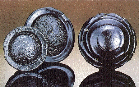
This process must be ongoing throughout the history of this sample, even after the deformation event and at lower temperatures. This is unequivocal evidence for pipe diffusion along a dislocation array in zircon, resulting in relatively fast and continuous redistribution of Pb over >10 μm [resulting in the production of nanospheres of pure metallic lead – see arrows in the photograph to the right]…
Reverse discordance has been the subject of a number of studies and is generally observed in high-U zircons (above a threshold of ~2,500 p.p.m. U). The phenomenon has been attributed to possible matrix effects, causing increased relative sputtering of Pb from high-U, metamict regions and resulting in a 1–3% increase in 206Pb/238U ages for every 1,000 p.p.m. U. However, in the zircon analysed here, the relationship between U content and reverse discordancy is not simple: several points show a degree of reverse discordance despite having U concentrations below 2,000 p.p.m., whereas the highest measured reverse discordancy (21%) is from a location with 3,102 p.p.m. U, only just above the threshold for which reverse discordancy is normally attributable to matrix effects. Different to analyses exhibiting some degree of reverse discordance, we interpret that the chemical signal of spot 2.8 represents a domain that is completely metamict. Although we cannot rule out some matrix effects in high-U, metamict zones, the complex relationship between U content and reverse discordancy in this zircon is further evidence for an additional process of Pb-enrichment—namely the pipe diffusion of Pb along dislocation arrays into adjacent metamict zones… Radiation damage may enhance this pipe diffusion/clustering behaviour…
Our results demonstrate the importance of deformation processes and microstructures on the localized trace element concentrations and continuous redistribution from the nanometre to micrometre scale in the mineral zircon… [and] have important implications for the use of zircon as a geochronometer, and highlight the importance of deformation on trace element redistribution in minerals and engineering materials… Dislocation movement through the zircon lattice can effectively sweep up and concentrate solute atoms at geological strain rates. Dislocation arrays can act as fast pathways for the diffusion of incompatible elements such as Pb across distances of >10 μm if they are connected to a chemical or structural sink. Hence, nominally immobile elements can become locally extremely mobile. Not only does our study confirm recent speculation that an understanding of the deformation microstructures within zircon grains is a necessity for subsequent, robust geochronological analyses but it also sheds light on potential pit-falls when utilizing element concentrations and ratios for geological studies.
Sandra Piazolo et. al., Deformation-induced trace element redistribution in zircon revealed using atom probe tomography, Nature Communications 7, Article number: 10490, doi:10.1038/ncomms10490 |Received | 31 August 2015 | Accepted | 18 December 2015 | Published | 12 February 2016 (Link)


Such factors can only contribute to the “preferential leaching” of various isotopes from zircons over time:
“238U decays via two very short-lived intermediates to 234U. Since 234U and 238U have the same chemical properties, it might be expected that they would not be fractionated by geological processes. However, Cherdyntsev and co-workers (1965, 1969) showed that such fractionation does occur. In fact, natural waters exhibit a considerable range in 234U/238U activities from unity (secular equilibrium) to values of 10 or more (e.g. Osmond and Cowart, 1982). Cherdyntsev et al. (1961) attributed these fractionations to radiation damage of crystal lattices, caused both by ” emission and by recoil of parent nuclides. In addition, radioactive decay may leave 234U in a more soluble +6 charge state than its parent (Rosholt et al., 1963). These processes (termed the ‘hot atom’ effect) facilitate preferential leaching of the two very short-lived intermediates and the longer-lived 234U nuclide into groundwater. The short-lived nuclides have a high probability of decaying into 234U before they can be adsorbed onto a substrate, and 234U is itself stabilised in surface waters as the soluble UO2++ ion, due to the generally oxidising conditions prevalent in the hydrosphere.” (Link)
Consider also that in a 2011 study, researchers led by geologist Birger Rasmussen of Curtin University in Bentley, Australia, analyzed more than 7000 zircons from a portion of the Jack Hills of Western Australia, where rocks are between 2.65 billion and 3.05 billion years old:
A total of 485 zircons held inclusions, and about a dozen or so of these contained radioactive trace elements that allowed the researchers to determine their ages. Those ages fell into two clumps—one of about 2.68 billion years and another of about 800 million years. “This was a big surprise to us,” Rasmussen says, especially because the zircons themselves ranged in age from 3.34 billion and 4.24 billion years old.
Rather than matching the ages of the zircons, the researchers note, the ages of the inclusions matched the ages of the metamorphic minerals surrounding the zircons. Some of those inclusions lie along hairline fractures in the zircons, a route by which mineral-rich fluids could have infiltrated, Rasmussen says. But other inclusions appear to be entirely enclosed. In those cases, the fluids may have traveled along defects in the zircon’s crystal structure caused by radioactive decay or along pathways that are either too small to see or oriented such that they’re invisible.
In recent years, some researchers have used analyses of zircons and their inclusions—and in particular, the temperatures and pressures they’ve been exposed to since their formation—to infer the presence of oceans or of modern-style plate tectonics on Earth more than 4 billion years ago, well before previously suspected, Rasmussen says. But based on the team’s new findings, which will be reported next month in Geology, those conclusions are suspect, he notes.
“This paper will stir people up,” says Ian Williams, an isotope geochemist at Australian National University in Canberra. “These results make it much less likely that Jack Hills zircons were involved in plate tectonics.” The team’s results “suggest that analyses of zircon inclusions can’t be trusted much at all,” adds Jonathan Patchett, an isotope geochemist at the University of Arizona in Tucson. “This is really nice work, very strong.” (Link)
Summary:
What this means is that:
- Zircon crystals are open systems that become more and more open over time in line with the degree of radioactive material that they contain and the corresponding radiation damage that takes place.
- Various isotopes, to include uranium and lead isotopes, can move around fairly rapidly within apparently “pristine” zircons – and probably back and forth between zircons and the surrounding igneous rock.
- Zircon dating methods are not independent and must be verified or calibrated against other radiometric dating methods.
- “Old zircons” can be incorporated into “new zircons” without a clear distinction.
- It seems then that such systems cannot be used as independently reliable clocks over long periods of time.
Cosmogenic Isotope Dating:

As another example, consider that 3H levels (from decay of a cosmogenic nuclide, 36Cl, produced by the interaction of cosmic rays with the nucleus of an atom) has been used to establish the theory that the driest desert on Earth, Coastal Range of the Atacama desert in northern Chile (which is 20 time drier than Death Valley) has been without any rain or significant moisture of any kind for around 25 million years. The only problem with this theory is that investigators have since discovered fairly extensive deposits of very well preserved animal droppings associated with grasses as well as human-produced artifacts such as arrowheads and the like. Radiocarbon dating of these finding indicate very active life in at least semiarid conditions within the past 11,000 years – a far cry from 25 million years. So, what happened?
 As it turns out, cosmogenic isotope dating has a host of problems. The production rate is a huge issue. Production rates depend upon several factors to include “latitude, altitude, surface erosion rates, sample composition, depth of sample, variations of cosmic and solar ray flux, inclusion of other radioactive elements and their contribution to target nucleotide production, variations in the geomagnetic field, muon capture reactions, various shielding effects, and, of course, the reliability of the calibration methods used.”
So many variables become somewhat problematic. This problem has been highlighted by certain studies that have evaluated the published production rates of certain isotopes which have been published by different groups of scientists. At least regarding 36Cl in particular, there has been “no consistent pattern of variance seen between each respective research group’s production rates” (Swanson 2001). To put it differently, “different analytical approaches at different localities were used to work out 36Cl production rates, which are discordant.” ( See also: CRONUS-Earth project, Link – last accessed March 2009)
In short, it doesn’t inspire one with a great deal of confidence in the unbiased reliability of cosmogenic isotopic dating techniques and only adds to the conclusion that different dating methods do not generally agree with each other unless they are first calibrated against each other.
Fission Track Dating:
 Overview:

Fission track dating is a radioisotopic dating method that depends on the tendency of uranium (Uranium-238) to undergo spontaneous fission as well as the usual decay process. The large amount of energy released in the fission process ejects the two nuclear fragments into the surrounding crystalline material, causing damage that produces linear paths called fission tracks. The number of these tracks, generally 10-20 µ in length, is a function of the initial uranium content of the sample and of time. These tracks can be made visible under light microscopy by etching with an acid solution so they can then be counted.
The usefulness of this as a dating technique stems from the tendency of some materials to lose their fission-track records when heated, thus producing samples that contain fission-tracks produced since they last cooled down. The useful age range of this technique is thought to range from 100 years to 100 million years before present (BP), although error estimates are difficult to assess and are rarely given. Generally it is thought to be most useful for dating in the window between 30,000 and 100,000 years BP.
A problem with fission-track dating is that the rates of spontaneous fission are very slow, requiring the presence of a fairly significant amount of uranium in a sample to produce useful numbers of tracks over time. Additionally, variations in uranium content within a sample can lead to large variations in fission track counts in different sections of the same sample.
Calibration:
Because of such potential errors, most forms of fission track dating use a form of calibration or “comparison of spontaneous and induced fission track density against a standard of known age. The principle involved is no different from that used in many methods of analytical chemistry, where comparison to a standard eliminates some of the more poorly controlled variables. In the zeta method, the dose, cross section, and spontaneous fission decay constant, and uranium isotope ratio are combined into a single constant.” (Link)
“Each dosimeter glass is calibrated repeatedly against zircon age standards from the Fish Canyon and Bishop tuffs, the Tardree rhyolite and Southern African kimberlites, to obtain empirical calibration factors ζ.” (Link)
“Zircon fission track ages, in agreement with independent K-Ar ages, are obtained by calculating the same track count data with each of the preferred values of λf (λf = 7.03 × 10⁻¹⁷yr−1 and 8.46 × 10⁻¹⁷yr−1) together with appropriate, selected neutron dosimetry schemes. An alternative approach is presented, formally relating unknown ages of samples to known ages of standards, either by direct comparison of standard and sample track densities, or by the repeated calibration of a glass against age standards.” (Link)
Of course, this means that the fission track dating method is not an independent method of radiometric dating, but is dependent upon the reliability of other dating methods – particular zircon-age standards usually derived from K-Ar, Ar-Ar, Rb-Sr, or U-Pb dating methods. The reason for this is also at least partly due to the fact that the actual rate of fission track production is debatable. Some experts suggest using a rate constant of 6.85×10⁻¹⁷ yr-1 while others recommend using a rate of 8.46×10⁻¹⁷ yr-1 (G. A. Wagner, Letters to Nature, June 16, 1977). This difference might not seem like much, but when it comes to dates of over one or two million years, this difference amounts to about 25-30% in the estimated age value. In other words, the actual rate of fission track production isn’t really known, nor is it known if this rate can be affected by various concentrations of U238 or other physical factors. For example, all fission reactions produce neutrons. What happens if fission from some other radioactive element, like U234 or some other radioisotope, produces tracks? Might not these trackways be easily confused with those created by fission of U238?
The human element is also important here. Fission trackways have to be manually counted. This is problematic since interpreting what is and what is not a true trackway isn’t easy. Geologists themselves recognize the problem of mistaking non-trackway imperfections as fission tracks. “Microlites and vesicles in the glass etch out in much the same way as tracks” (Link). Of course, there are ways to avoid some of these potential pitfalls. For example, it is recommended that one choose samples with as few vesicles and microlites as possible. But, how is one to do this if they are so easily confused with true trackways? Fortunately, there are a few other “hints”. True tracks are straight, never curved. They also tend to show characteristic ends that demonstrate “younging” of the etched track. True tracks are thought to form randomly and have a random orientation. Therefore, trackways that show a distribution pattern tend not to be trusted as being “true”. Certain color and size patterns within a certain range are also used as helpful hints. Yet, even with all these hints in place, it has been shown that different people count the same trackways differently – up to 20% differently (Link). Add up the human error with the error of fission track rate and we are suddenly up to a range of error of 50% or so.
Consider also that In 2000, Raymond Jonckheere and Gunther Wagner (American Minerologist, 2000) published results showing that there are two kinds of real fission trackways that had “not been identified previously.” The first type of trackway identified is a “stable” track and the second type is produced through fluid inclusions. As it turns out, the “stable tracks do not shorten significantly even when heated to temperatures well above those normally sufficient for complete annealing of fission tracks.” Of course, this means that the “age” of the sample would not represent the time since the last thermal episode as previously thought. The tracks through fluid are also interesting. They are “excessively long”. This is because a fission fragment traveling through a fluid inclusion does so without appreciable energy loss. Such features, if undetected, “can distort the temperature-time paths constructed on the basis of confined fission-track-length measurements.” Again, the authors propose measures to avoid such pitfalls, but this just adds to the complexity of this dating method and calls into question the dates obtained before the publication of this paper (i.e., before 2000).
Add up all of these potential pitfalls and it becomes quite clear as to why calibration with other dating techniques is required in fission track dating. It just isn’t very reliable or accurate by itself. Generally speaking, then, it is no wonder that fission-track dating is in general agreement with Potassium-Argon dating or Uranium-Lead dating on within a given specimen – since the calibration of fission track dating would almost force such agreement.
However, there are still several interesting contradictions, despite calibration. For example, Naeser and Fleischer (Harvard University) showed that, depending upon the calibration method chosen, the calculated age of a given rock (from Cerro de Mercado, Mexico in this case) could be different from each other by a factor of “sixty or more” – – “which give geologically unreasonable ages” (Link).
“In addition, published data concerning the length of fission tracks and the annealing of minerals imply that the basic assumptions used in an alternative procedure, the length reduction-correction method, are also invalid for many crystal types and must be approached with caution unless individually justified for a particular mineral” (Link).
Now that’s pretty significant – being off by a factor of sixty or more? No wonder the authors recommend only going with results that do not provide “geologically unreasonable ages”.
Tektites:
 Another example of this sort of error with fission track dating comes in the form of glass globs known as “tektites”. Tektites are thought to be produced when a meteor impacts the Earth. When the massive impact creates a lot of heat, which melts the rocks of the Earth and send them hurtling through the atmosphere at incredible speed. As these fragments travel through the atmosphere, they become super-heated and malleable as they melt to a read-hot glow, and are formed and shaped as they fly along. It is thought that the date of the impact can be dated by using various radiometric dating methods to date the tektites. For example, Australian tektites (known as australites) show K-Ar and fission track ages clustering around 700,000 years. The problem is that their stratigraphic ages show a far different picture. Edmund Gill, of the National Museum of Victoria, Melbourne, while working the Port Campbell area of western Victoria uncovered 14 australite samples in situ above the hardpan soil zone. This zone had been previously dated by the radiocarbon method at seven locales, the oldest dating at only 7,300 radiocarbon years ago (Gill 1965). Charcoal from the same level as that containing specimen 9 yielded a radiocarbon age of 5,700 years. The possibility of transport from an older source area was investigated and ruled out. Since the “Port Campbell australites include the best preserved tektites in the world … any movement of the australites that has occurred … has been gentle and has not covered a great distance” (Gill 1965). Aboriginal implements have been discovered in association with the australites. A fission-track age of 800,000 years and a K-Ar age of 610,000 years for these same australites unavoidably clashes with the obvious stratigraphic and archaeological interpretation of just a few thousand years.
“Hence, geological evidence from the Australian mainland is at variance, both as to infall frequency and age, with K-Ar and fission-track dating” (Lovering et al. 1972). Commenting on the above findings by Lovering and his associates, the editors of the book,Tektites, state that, “in this paper they have built an incontrovertible case for the geologically young age of australite arrival on earth” (Barnes and Barnes 1973, p. 214).
This is problematic. The argument that various radiometric dating methods agree with each other isn’t necessarily true – especially when organic remains that can be Carbon-14 dated are available. Here we have the K-Ar and fission track dating methods agreeing with each other, but disagreeing dramatically with the radiocarbon and historical dating methods (which is not an uncommon situation). These findings suggest that, at least as far as tektites are concerned, the complete loss of 40Ar (and therefore the resetting of the radiometric clock) may not be valid (Clark et al. 1966). It has also been shown that different parts of the same tektite have significantly different K-Ar ages (McDougall and Lovering, 1969). This finding suggests a real disconnect when it comes to the reliability of at least two of the most commonly used radiometric dating techniques (Link).
In short, it seems like fission track dating is tenuous a best – even as a relative dating technique that must first be calibrated against other dating techniques.
Carbon 14 Dating:
Introduction:
 All living things on this planet are built upon a carbon backbone so to speak. Carbon is one of the key elements that makes life, as we know it, possible. So, during the lifetime of any living thing, carbon is taken in and used as part of the building blocks of the body of the organism. Since various isotopes of carbon are chemically indistinguishable, both carbon-12 (stable) and carbon-14 radioactive (produce when cosmic rays turn nitrogen-14 in to carbon-14) will both be equally in proportion to the existing ratios of these isotopes within the environment at the time. And, this ratio will be maintained within the tissues of the organism for its entire life. However, when the organism dies, the carbon contained within its tissues not longer interact with the carbon within the surrounding environment. So, the ratio of 12C vs. 14C will increase over time because of the radioactive decay of 14C back into 14N with a relatively short half life of 5730 years.
So, given the ratio of atmospheric 14C to 12C one can determine the time of death of a given organism by measuring the remaining amount of 14C within the tissues of the organisms and comparing that amount to the original amount (i.e., the amount that was present within the atmosphere).
Calibration:
 It all seems rather straightforward. However, there are a few caveats. For example, the ratio of atmospheric 14C to 12C doesn’t stay the same over time, but changes. Also, there are regional variations in the ratio that must be considered. This is why carbon-14 dating isn’t an entirely independent dating method, but requires calibration against other dating methods – like various historically-derived events and tree-ring dating for instance (Link). Of course, tree ring dating is in turn calibrated by other dating techniques, primarily carbon-14 dating – which is just a bit circular. Also, attempts to use amino acid racemization rates as a dating method with efforts to help to calibrate radiocarbon dating have failed. AAR dating methods have themselves also turned out to require calibration by radiocarbon dating (Link).
Dinosaur Soft Tissue Preservation:

As a related concept, consider the fairly recent discovery of original soft tissue remains within the bones of numerous dinosaurs thought to be more than 60 million years old (Link) – soft tissue that maintained flexibility and elasticity as well as cellular structure and original antigenic activity (based on fairly large intact portions of proteins and even fragments of DNA). By itself, this finding was completely unexpected from the evolutionary perspective since it was long argued that soft tissues and proteins (even fragments of DNA) could not be maintained longer than 100,000 years or so due to the problem of kinetic chemistry where such organic molecules self-destruct (because of their constant movements/vibrations) over relatively short periods of time at ambient temperatures.
 As far as the various factors that might impact soft tissue, protein and DNA decay over time, certainly various studies have taken many of these into account – to include temperature (which seems to be the primary factor in setting the rate of decay), as well as pH, amino acid composition of the protein, water concentration of the environment, size of the macromolecule, ionic strength of the environment, cross linking or covalent bonding within the molecules (as in the case of formaldehyde or iron preservation), etc. Of course there could be other as yet unknown factors that might contribute to protein/DNA preservation. However, these have yet to be found as far as I’m aware – at least not to the point of explaining how tens of millions of years of protein/DNA preservation could tenably be achieved.
For example, Allentoft, M.E. et al. (2012) argued that no intact DNA bonds can be expected at 22,000 years at 25°C, 131,000 years at 15°C, 882,000 years at 5°C; and even if it could somehow be kept continually below freezing point at –5°C, it could survive only 6.83 Ma. Basically, DNA has about a “521 year half-life” (Link).
“Even under the best preservation conditions at –5°C, our model predicts that no intact bonds (average length = 1 bp [base pair]) will remain in the DNA ‘strand’ after 6.8 Myr. This displays the extreme improbability of being able to amplify a 174 bp DNA fragment from an 80–85 Myr old Cretaceous bone.”
 And, this statement was published well after Schweitzer made her discoveries of fragments of protein and DNA within dinosaur soft tissues. This statement is also interesting because dinosaur bones are generally believed to have experienced greater than 20°C temperatures for tens of millions of years (Buckley, et al., 2008).
Other features, such as rapid desiccation and high salt concentrations, may also prolong DNA survival (Lindahl 1993). However, kinetic calculations still predict that small fragments of DNA (100–500 bp) will survive for no more than 10 kyr in temperate regions and for a maximum of 100 kyr at colder latitudes (Poinar et al. 1996; Smith et al. 2001).
 And, the half-life for the average protein is similar since the “peptide bond has a half-life of 400 years” (Adv Exp Med Biol. 2009; 611: xci–xcviii). However, some proteins, such as collagen in particular, appear to have somewhat longer half-lives of ~2,000 years at ambient temperatures (Buckley, et al., 2008).
And yet, sizable fragments of both DNA and antigenic proteins have been found within dinosaur soft tissue remains. The minimum requirement for antibody binding to DNA is that about 35-40 bp remain intact – which were in fact discovered in dinosaur soft tissues by antigen binding by Mary Schweitzer (Link). And, this isn’t the first time that DNA fragments have been detected in dinosaur bones. In fact, according to Jack Horner, “Getting DNA out of [dinosaur] bones is easy. We have the same thing Woodward has [Link]–we have DNA [to include fragments up to 174bp, ironically, which were sequenced by Woodward in 1994 who still believes these fragments to be dinosaur DNA despite all the controversy], but we  can’t prove that it’s from a dinosaur… If we find these proteins [which have been found and sequenced since this 1995 interview with Horner] it will be much more convincing that we have dinosaur DNA” (Link). Add to this that Dr. Svante Paabo of the University of Munich said, “We have found that the DNA of insects preserved in amber for many millions of years has survived with surprisingly little degradation.” (Link)
In short, there is pretty good evidence that reasonably-sized fragments of DNA have in fact survived within the soft tissues of dinosaur bones and other creatures – fragments that are comparable in size to those detected in Pleistocene animal remains…
Carbon 14 in Dinosaur Soft Tissues:
However, beyond this little conundrum, it has also been shown that such soft tissues contain significant quantities of radiocarbon (14C). Surprisingly, 14C has actually been discovered in the soft tissues of many dinosaur bones examined thus far, producing ages ranging from 16,000 to 32,000 years before present – essentially the same as the radiocarbon ages reported for large Pleistocene mammals such as mammoths, mastodons, dire wolves, etc. (Link, Link). Also, pretty much all coal samples contain fairly significant quantities of radiocarbon.
What is especially interesting about carbon-14 is that, once an organism dies, the 14C that was in that creature at the time of dead does not leave. It stays there until it decays back into 14N. This is a distinct advantage over many of the other radiometric dating techniques where parent and/or daughter elements can escape into the surrounding environment over time. Also, there is no good way to incorporate 14C into the tissues of a dead organism – outside of bringing in foreign organic material or producing 14C in situ from the radioactive decay of closely associated radioactive materials (such as uranium).
This is important to keep in mind because essentially no detectable 14C should exist within the remains of a dead organism after 100,000 years – because of the relatively short half-life on 14C. So, if any detectable level of 14C is discovered in the remains of a dead organism, it is reasonable to conclude that the organism died within the last 100,000 years.
The usual counterarguments of either contamination or in situ production don’t hold water when it comes to explaining the very high levels of radiocarbon so consistently and generally found throughout the fossil record (Link, Link, Link).
Catastrophic Decrease in Historical Levels of Carbon-12:
 Suppose there had been a major atmospheric disturbance, such as the one described in the flood “myths” of many diverse cultures about 5,000 years ago. If true, might such a global catastrophe be expected to alter the 14C to 12C ratio just a little bit? Perhaps, but by how much and would this really be significant?
Consider, for argument’s sake, what would happen to the carbon-14 dating assumptions if there was a significantly greater quantity of carbon 12 in the biosphere of this earth sometime in the recent past. What would this do to the 14C to 12C ratio? Obviously, it would be reduced. This reduction in the 14C to 12C ratio would give an increased apparent age compared to today’s ratio.
Now, what happens if the geologic column and the fossil record really are records of truly catastrophic processes? As it turns out, there are around 39 trillion metric tons of carbon in the biosphere. However, there are around 6,820 trillion metric tons of carbon currently buried in the form of coal, oil, and fossils. This is about 175 times the amount of organic matter than we have living today. What if this buried organic material was all actually part of the biosphere at the same time? Sedimentary carbonates are a huge block of carbon to consider, as much as 20,000 trillion metric tons of sedimentary carbonates are found in the geologic column. What if some of this carbon (12C) was also part of the biosphere at the same time? Then, what if this huge mass of living organisms were suddenly buried rapidly in some catastrophic calamity? If true, this would mean that the amount of carbon-12 in and available to the biosphere was significantly greater in the past than it is today. In fact, without even considering the carbon in the vast quantities of calcium carbonate, there is enough carbon 12 buried in the fossil coal, oil, and other fossils to reduce the apparent ratio of 14C to 12C by about 7 half-lives. (Link)
So, unless the production of carbon-14 was equally greater in the past (either via markedly increased nitrogen 14 and/or radiation), such a huge and sudden loss of carbon-12 from the biosphere would dramatically increase the ratio of 14C vs. 12C (equivalent to about 7 half lives). Obviously then, this would completely throw off the whole basis of carbon-14 dating going farther back in time beyond such a catastrophic event or a closely-spaced series of catastrophic events. Certainly then, carbon-14 could not be used to rule out the recent occurrence of such a global catastrophe.
There is also what is called a “reservoir effect” where significant variations of the ratio of present day 14C to 12C are recognized (as compared to the average ratio in the overall biosphere). Since the oceans have lower levels of carbon 14 compared to the atmosphere, most living marine creatures date at least several hundred years old. Also, because of local thermal vents that spew out large quantities of carbon-12, certain aquatic mosses living in Iceland date as old as 6,000 to 8,000 years via the carbon-14 dating method. And, in Nevada, living snails have apparent carbon-14 ages up to 27,000 years old. Marine shells in Hawaii show younger dates if preserved in volcanic ash vs. limestone. (Link) Also, research has shown the ancient peat reveals an marked decrease in carbon-14 ratios at lower and lower levels (i.e., decreased carbon-14 with older age well beyond what would be expected with radioactive decay and therefore more consistent with a Noachian-style catastrophe within fairly recent history) (Link).
Assuming A Literal Creation Week and a Noachian-Style Flood:
Now, just suppose, for argument’s sake, that we take the claims of the biblical authors seriously and consider what we should expect given a literal 7-day creation week and an enormous world-wide Noachian-style flood within fairly recent history (i.e., less than 10,000 years go). What would we expect to see in our world today? Here are a few potential observations that come to mind:
Before the Flood:
 In order to be able to make a comparison between the pre- and post-Flood worlds, we need to consider what the world was like before the Flood. According to the Bible and the writings of Mrs. White, before the biblical Flood, there were no great oceans, mountain ranges, or deserts. The Earth was watered by underground springs and fountains driven by four great rivers (Genesis 2:10). The ground was watered by dew each morning, so there was no need for rain. In fact, it never rained. That is why Genesis described the inhabitants of the pre-Flood world as laughing at Noah when he said that water would soon fall from the sky and flood the world. Such a thing was a scientific impossibility in that day – that was until all of the fountains of the great deep were broken up within a single day (Genesis 7:11).
 Consider also that there were no great mountain ranges, oceans, or ocean trenches because there were no “continents” or “continental plates” or “continental drift”. If the crust of the Earth were broken up within a single day (likely by impacts from massive asteroids/meteors), the continental “plates” would have been formed on that day as well – like a cracked egg. The massive release of energy associated with this event would have initially driven very rapidly continental drift. As the continents began to move rapidly relative to each other, mountain ranges and ocean trenches would have formed at a fairly rapid initial rate, using up significant amounts of energy in the process. So, like two cars in a crash, the initial formation of mountain ranges and trenches would absorb much of the initial energy, rapidly reducing the rate of continental drift as well as the formation of
 mountains and ocean trenches so that today’s rate of drift and orogeny (or mountain building) would be much much slower in comparison. The same would be true of volcanic activity. Before the Flood, there were no volcanoes. However, during the initial development of the Flood and associated catastrophic break up of the Earth’s crust, volcanic activity would have been massive all around the world – especially along the major fault lines, but would then have tapered off over time (which is what we see in the geologic record with far more massive volcanoes and volcanic activity in the past compared to today’s situation – or anything within the memory of mankind outside of the Bible or various legends of an ancient world-wide catastrophe of Noachian proportions).
 Such heavy volcanic activity would have extruded far more radioactive material than had ever existed on the surface of the Earth before the Flood. In fact, it is the radioactive elements that maintain the molten nature of the Earth’s core. Without these elements, the Earth’s core would cool off much more rapidly and the Earth would then become a dead planet like Mars (Mars once had a strong magnetic field—like Earth does now—produced by a dynamo effect from its interior heat).
Lord Kelvin and the Age of the Earth:
 For example, Lord Kelvin originally estimated the ages of both the Earth and the Sun based on cooling rates. The answer of “25 million years” deduced by Kelvin for the age of the Earth was not received favorably by geologists – since much more time was needed to adequately support Darwin’s theory of evolution. As one answer to his critics, Kelvin produced a completely independent estimate — this time for the age of the Sun. His result was in close agreement with his estimate of the age of the earth. The solar estimate was based on the idea that the energy supply for the solar radioactive flux is gravitational contraction. These two independent and agreeing dating methods for of the age of two primary members of the solar system formed a strong case for the correctness of his answer within the scientific community (This just goes to show that just because independent estimates of age seem to agree with each other doesn’t mean that they’re correct – despite the fact that this particular argument is the very same one used to support the validity of radiometric dating today. Other factors and basic assumptions must also be considered).
Of course, Kelvin formed his estimates of the age of the Sun without the knowledge of fusion as its true energy source. Without this knowledge, he argued that,
“As for the future, we may say, with equal certainty, that inhabitants of the Earth cannot continue to enjoy the light and heat essential to their life, for many million years longer, unless sources now unknown to us are prepared in the great storehouse of creation.”
This last statement proved prophetic. There were indeed powerful and unknown sources of energy fueling the Sun’s energy output.
Of course, the same is true of the basis of Kelvin’s estimate of the age of the Earth. Kelvin’s error was due to his idea that no significant source of novel heat energy was affecting the Earth. He believed this even though he did admit that some heat might be generated by the tidal forces or by chemical action. However, on the whole, he thought that these sources were not adequate to account for anything more than a small faction of the heat lost by the Earth. Based on these assumptions his finally estimate of the maximum age of the Earth was less than 10 Ma – which would have been a very reasonable conclusion save for the energy that is being created by radioactive decay within the molten layers of the Earth”s core.
Increased Radioactive Elements on the Surface of the Planet:
 When the crust of the Earth was broken up during the Flood, massive volcanic activity would have allowed these radioactive elements to be deposited on the surface of the Earth. For example, most uranium mines around the world are associated with mountainous/volcanic regions where the deformities in the Earth’s crust are most pronounced.
Of course, massive volcanoes were going off during the height of the Flood with much of the volcanic material being deposited under water and within water-deposited sedimentary layers. This means that this volcanic material, deposited under water or within thick layers of sediment, would have retained increased amounts of argon gas, thus falsely increasing the apparent K-Ar age of the volcanic material.
Also, at the same time, the rapid burial of massive amounts of organic material (and therefore of carbon-12) would have significantly increased the apparent carbon-14 age of the buried remains – compared to today’s C14/C12 ratio.
Where did All the Water Come From? and Go?
 Many wonder where on Earth all the water that would be required to produce a Noachian-style Flood might have come from? – and where did it go? After all, the Bible claims that the level of water rose so that all of the highest mountains of the day were covered by more than 20 feet (Genesis 7:20). Even if the mountains before the flood were relatively humble, it would still seem to take an enormous amount of water to cover the entire globe to such a depth. However, there are a few things to consider along these lines. First off, if there were no great ocean basins or great mountain chains before the Flood, the amount of water that is currently in the oceans would easily cover the entire globe to substantial depths.
 Beyond this, however, a 2014 an article was published in the journal Science by Brandon Schmandt et. al., arguing that massive amounts of water exist some 400 miles deep under our feet amounting to around three times the volume of all the world’s oceans (Link). These oceans of water have been locked within a sponge-like crystalline material called “blue ringwoodite.” To put this into perspective, consider that the crust of the Earth is only about 3-5 miles (8 kilometers) thick under the
  oceans (oceanic crust) and about 25 miles (32 kilometers) thick under the continents (continental crust). Despite the depth of this massive amount of water, consider what would happen if the Earth were to be hit by a huge asteroid. The sudden compression of the ringwoodite around the globe would cause it to release huge volumes of water. Under the immense pressure, this water would burst with great violence and velocity through cracks and great chasms in the Earth’s crust. Then, the pressure from the initial impact had subsided, the water would gradually be reabsorbed.
“We should be grateful for this deep reservoir,” says Jacobsen [a co-author of the study]. “If it wasn’t there, it would be on the surface of the Earth, and mountain tops would be the only land poking out.” (Link).
Bioturbation:
 During the Flood the massive tidal waves traveling rapidly around and around the world would have eroded and laid down massive amounts of sediments in sequential layers – quite rapidly. In fact such layers would have been laid down so rapidly that there would have been very little time for the normal processes that usually affect sedimentary flood deposits to affect the layers deposited by the Noachian Flood. Consider, for example, that after modern floods the sedimentary layers that are deposited are rapidly colonized by burrowing creatures that dig into and burrow through the various sedimentary layers – mixing them up over time. What happens, then, is that over a couple years or so the lines between the various layers of sediment become so mixed up by these burrowing organisms that they are completely homogenized and no longer distinguishable as individual layers of sediment. This process is called, “bioturbation”. Yet, this is not what is generally seen within the geologic column/fossil
  record. The layers within the geologic column are generally very well defined all around the world – with relatively little evidence of the expected bioturbation that should be seen if these layers had in fact been deposited with vast periods of time elapsing between the deposition of each layer.
 In October of 2009 and again in November of 2014, Dr. Arthur Chadwick from Southwestern Adventist University, gave some talks at Loma Linda University (see video below). During these talks Chadwick argued that if the strata of the geologic record had been laid down that slowly, in normal ecological conditions, we would expect bioturbation to effectively erase the evidences of aqueous deposition – such as particle sorting and bedding planes. But for the most part these features have not been erased and very little and often no bioturbation can be identified within the layers.
This feature, in particular, is much more consistent with a relatively rapid, even catastrophic, deposition of most of the layers of the geologic column/fossil record. In fact, the layers were laid down so fast and so deep that the usual effects of bioturbation were minimized – allowing for the preservation of the details particle sorting and bedding planes for the layers in the geologic record. In comparison, such evidence is very hard to explain as very slow or gradual deposition over hundreds of millions of years.
Warm world:
 Right after the Flood, of course, the world would have been a rather warm place because of all the energy released during the catastrophe. There were no ice caps on the poles since even within the Arctic Circle it was warm and lush all around the world, harboring enormous forests and fruit bearing trees as well as vast grasslands and millions of animals – to include large mammoths, dear, bison, etc. This situation lasted for hundreds of years after the Flood. However, when the first ice-age came, it came so suddenly that it trapped, froze, and preserved millions of these trees and animals all around the Arctic Circle. This means, of course, that Greenland was also once very green – in very recent history.
Greenland was once Green:
 Greenland, in particular, has not always been covered in ice. It was once truly green – all over. In fact, within the Hypsithermal period or “warm age” (which, according to mainstream thinking, is said to have lasted some 7,000 years, ending only some 2,500 years ago), the northernmost parts of the planet were very much warmer than they are today. Studies on sedimentary cores carried out in the North Atlantic between Hudson Strait and Cape Hatteras indicate ocean temperatures of 18°C (verses about 8°C today in this region) during the height of this period of time between 4,000 to 6,000 years ago (again, according to mainstream thinking). Given that the Greenland ice sheet is currently melting at a fairly rapid rate, it’s rather hard to believe that it existed at all during the very warm Hypsithermal period – a period when millions of mammoths along with many other types of warmer weather plants and animals happily lived within the Arctic Circle all around the globe along the very same latitudes as Greenland (Link). A 1995 study of mammoth remains located on Wrangel Island (on the border of the East-Siberian and Chukchi Seas) shows, according to radiocarbon dating, that mammoths persisted on this island till about 1,700 B.C. (Vartanyan S.L, et. al., 1995). And yet, somehow, Greenland was still covered with thick sheets of ice that are over 400,000 years old (Link), when everything around it was warm and balmy? supporting huge herds of animals and lush forests with fruit bearing trees and abundant grasslands? This seems quite unlikely to me…
More at: Ancient Ice
World-wide Paleocurrents:

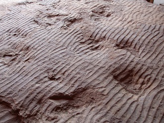 Consider also that the sudden release of energy that cause the break-up of the Earth’s crust, continental drift, and the building of massive mountain ranges and ocean trenches, would have produced many huge tsunamis hundreds or even thousands of feet tall traveling at hundreds of miles per hour around the globe, eroding and depositing massive amounts of sediment with each pass. Traces of the direction of these massive waves and the general movements of the water that laid down the sediment should still be visible today – and they are. Most sedimentary layers around the world have ripple marks along their surfaces, indicating the direction of water flow, or the “paleocurrent” that laid down each layer. And, interestingly, the directly of water flow is consistent, all around the world, for various layers within the lower layers of the geologic column (especially the Paleozoic layers). These continental, or even worldwide paleocurrents, all showing a general pattern for a given series of layers (Link) are much easier for a rather sudden catastrophic Flood model to explain compared to the standard uniformitarian model of slow geologic evolution over millions of years. It is also consistent with the idea that, before the Flood, there were no long chains of very high mountains. Otherwise, such continent-wide paleocurrents could not have been produced.
Paleocurrents change pattern and general direction within different levels of the geologic column at different places around the globe. However, if you watch Dr. Giem’s video presentation and look at all of the maps presented on Chadwick’s website it seems an unavoidable conclusion that continent wide patterns emerge that even involve multiple continents.

As Chadwick points out, “During the Paleozoic, in sharp contrast to Mesozoic, Cenozoic and Precambrian tendencies, clear and persistent continent-wide trends are normative. Sediments moved generally from east and northeast to west and southwest across the North American Continent. This trend persists throughout the Paleozoic and includes all sediment types and depositional environments. A gradual shift is seen from lower and mid Paleozoic westerly trends to upper Paleozoic southerly trends… Paleozoic paleocurrents indicate the influence of directional forces on a grand scale over an extended period. Various authors have attributed the directionality to such things as “regional slopes,” but it is difficult to see how this could apply to deposits of such diverse origins over so wide an area. The lack of strong directionality in the underlying Precambrian sustains the need to seek understanding of what makes the Paleozoic style of sedimentation unique with respect to directional indicators.” (Link).
This is consistent with the start of the Flood and the initial impacts that broke up the Earth’s crust “within a single day”, starting at the beginning of the Paleozoic – and then tapering off as the Flood proceeded and became more and more complex in nature (with additional meteor strikes, rapid continental separation and drift and mountain building).
This concept is further confirmed by finding sediments that appear to have been transported clean across entire continents. Consider the following example:

The Navajo Sandstone of southern Utah [Jurassic], best seen in the spectacular mesas and cliffs in and around Zion National Park, is well above the Kaibab Limestone, which forms the rim rock of the Grand Canyon. It was once thought to have been formed as desert dunes in an ancient desert like the Sahara Desert. Subsequently, however, it has been determined that these sand “dunes” were actually formed under water and that the sand itself was transported across the entire country from the Appalachians of Pennsylvania (based on grains of zircon crystals that contain uranium similar in character to those of the Appalachians). If this is true, the sand grains were transported at least 1,800 miles (3000 km) right across North America. And, the evidence is overwhelming that the water was flowing in one general direction to carry this much sediment across the entire continent. More than half a million measurements have been collected from 15,615 North American localities, recording water current direction indicators throughout the geologic record. The evidence indicates that water moved sediments across the entire continent, from the east and northeast to the west and southwest throughout the Paleozoic. This general pattern continued on up into the Mesozoic, when the Navajo Sandstone was deposited. How could water be flowing across the North American continent consistently for hundreds of millions of years in some complex river system for which no evidence exists? These findings seem to be much more consistent with massive sheets of water from a Noachian-style Flood.
As far as the underwater origin of the Navajo dunes: “A 1975 study by scientists Freeman and Visher (Journal of Sedimentary Petrology, 45:3:651-668) provides some important insights as to the origin of the Navajo Sandstone [Link]. The investigators pointed out that underwater sand dunes are known to accumulate on portions of the sea floor swept by strong currents–for example, beneath the North Sea. Superficially they look a lot like desert (windblown) sand dunes, but careful analysis of their grain size distribution reveals major differences. It turns out that disaggregated sands from the Navajo Sandstone match very well with modern submarine dunes, and very poorly with desert dunes. If the Navajo Sandstone formed underwater, as the data seem to indicate, then one must imagine water depths on the order of 300 feet and current velocities of 4 feet per second across large portions of North America! [Leonard Brand also cited this evidence for the under-water formation of the Navajo Sandstone; Link].
Freeman and Visher also observed a bedform called “current lineation,” which so far has been found only in marine dunes. Furthermore, folds in the Navajo Sandstone indicate that thicknesses in excess of several hundred feet were in a water-wet and unconsolidated state at the same time. This too suggests rapid underwater burial.” (Link)
So, now there are two independent lines of evidence (paleocurrents and sediment transport) pointing in the same direction…
Lack of Ocean Sediment:
Ocean sedimentation, or the lack thereof, is also a big problem for the neo-Darwinian perspective as well. There simply isn’t enough of it – not by a long shot. Consider that if Pangea really did split apart some 200 million years ago that the ocean basin should be completely filled with sediment by now.
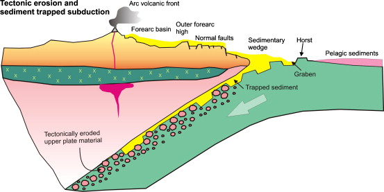 How is that? Well, around 30 billion tons of sediment per year are carried into the oceans by continental erosion. Subduction by plate tectonics only removes ~2.5 billion tons per year. That leaves an excess of 27.5 billion tons of sediment per year to build up within the ocean basins. Currently, only 1e17 tons of sediment exist within the ocean basins. Yet, this tonnage could be deposited within just 15 million years. Given that the oceans are supposed to be some 3 billion years old, where did all the extra tonnage go?
According to Alexander Lisitzin (1996) the problem is even worse. His calculations show that there are only around 133 million Km3 of sediment in the oceans today while 18 Km3 of sediment is being deposited per year (and only 1.5 Km3 is being subducted annually). This works out to be around 8 million years worth of sediment within the oceans today (Link).
Common Counterarguments:
So, again, what happened to the rest of the sediment? – enough sediment to completely fill in the oceans many times over? A common counter argument I often here goes as follows:
This is a disingenuous ‘proof’ that overlooks some fundamental facts. One is that the rate of deposition is not constant. When the Earth was young and consisted of hard, igneous rock, there was very little deposition. When some of the hard, igneous rock became overlaid with softer, secondary rock, erosion increased. Much of present-day erosion is not even erosion of rocks – it is erosion of soils that were laid down in the much more recent past and which are removed relatively quickly (Link).
The problem with this argument is that there is no rational reason to believe that current erosion rates (annual averages) where significantly different in the past than they are today – at least not nearly enough to make up for the problem. In fact, there are arguments that during the past 30 Ma annual global erosion rates were actually higher, on average, than they are today (because of humans building large dams, blocking large rivers, and preventing the usual levels of sediment that they carry to reach the oceans).
Along these lines, if one is going to argue for the value of deep ocean sediment cores to tell us something about the past:
“Direct measurements of sedimentation rates in deep-drilled sequences show that sedimentation rates in the past were of the same order as the present rates.”
– Alexander Lisitzin (1996), Oceanic Sedimentation: Lithology and Geochemistry.
And, after all, we’re only talking 15 Ma to produce the current sediment in the oceans. That’s a drop in the bucket from the Darwinian perspective. Certainly erosion rates are not thought to have been significantly different a few tens of millions of years ago vs. today. Consider also that volcanic rock isn’t that resistant to erosion and the mountain ranges around the world supposedly started their uplift some 50-70 Ma – mountains that are still covered by sedimentary rock today (even though it should have been washed off many times over by now).
Now, I’ve often heard the argument that farming and agriculture have significantly increased the erosion rate. However, as already mentioned, this increase has been effectively compensated for by the river dams that have been built worldwide.
Here are a few other counter arguments I’ve heard along the way:
Another fact that creationists prefer to overlook is that the sediment does not remain as sand or mud. Deep layers of sand on the ocean floor are under immense pressure and turn into sandstone. Mud may turn into shale, and so on. Even if these secondary rocks remained on the ocean floor, it would simply mean that the oceans would sit on top of the new floor. Easy. (Link)
The sediment estimate I listed accounts for this. Even with the “mud turned to sandstone” argument, there doesn’t seem to be enough sediment in the oceans to make up the difference – not by a long shot.
But the secondary rocks do not stay on the ocean floor – that is why we have many of our non-igneous rocks that are now on dry land. Continental drift and geological uplifting is constantly changing the shape of the Earth – raising up new mountain ranges and pushing up parts of the sea bed high above the water level, while lowering others. Even creationists admit that these forces exist, although they try to minimise their duration. (Link)
Of course mountain uplifts and trenches are formed. So what? How does this explain the lack of sediments in the vast oceans? Somehow it all got uplifted out? Really?
There is some of your supposed sediment that is missing from the oceans – making the Himalaya.
This severely underestimates the degree of the problem at hand.
During a period of one billion years around 30 billion billion tons of sediment would be deposited in the oceans – at current rates. This is enough to cover the entire ocean floor with a thickness of almost 20 miles of sediment. Since the oceans are quite a bit larger than the dry landmass of the planet, this means that a thickness of almost 40 miles of sediment would need to have been washed off the continents.
Mt. Everest (only about 5.5 miles tall) is currently covered by Ordovician limestone that was supposedly deposited some 440-480 million years ago.
The removal of the sediment from the oceans on the tops the continents and mountains around the world is the tiniest drop in the bucket compared to the amount of sediment that would have reasonably been deposited into the oceans during those hundreds of millions of years.
The Himalayan mountains, in particular, are supposed to have started their uplift some 50 Ma. Since that time, three times the sediment should have been deposited into the oceans compared to what currently exists in the oceans. Forget about the notion that the oceans are supposed to be ~3 billion years old. Even the ocean floor that was produced by continental drift since Pangea (supposedly 200 Ma ago) is practically devoid of sediment. Why is that? – given any reasonable measure of expected sedimentation rates?
So the evolutionists, with their measurements of radiation, magnetism, fossils, etc. have a remarkably good story for how this whole shape comes about – something completely lacking in the YEC/YLC community.
How is this a “remarkably good” explanation when it comes to the continued existence of sedimentary layers on the tops of these steep mountains for tens of millions of years? or when it comes to explaining the lack of ocean sediments? Neither of these questions are even addressed much less tenably answered.
Lack of Erosion:
 The existence of sediments on top of huge mountain ranges is itself a huge mystery from the Darwinian perspective. An erosion rate of 200 cm/kyr is about average for the Himalayan region given the newer estimates based on 10Be and 26Al measurements, which suggest an average erosion rate of the Himalayas of 130 cm/kyr for the lower altitudes and up to 410 cm/kyr for the steepest areas with an average in the high Himalayas of about 270 cm/kyr (see cross section of the Himalayan Mountains).
Basically, the Ordovician limestone has been exposed to high-level high-altitude erosion (~200 cm/kyr) for at least 20 million years? – and it is still there? How then can Mt. Everest really be over 50 million years old, or even 20 million years old and still have a Ordovician layer of sediment covering it as if it had hardly been touched by erosion?
 Some mountain ranges, such as the Chugach and St. Elias mountain ranges in southeast Alaska, are currently eroding at “50 to 100 times” the current Rocky Mountain rate – i.e., at about 5,000 to 10,000cm/kyr or 50,000 to 100,000 meters of erosion per million years.
Such erosion cannot be rationally explained by arguing that somehow such rates where much much less in the past than they are today. There is simply is no rational explanation for this conclusion that I’ve been able to find. After all, according to mainstream geologists the last 30 Ma in particular had higher average rates of annual erosion compared to today’s rates.
At the current rate of erosion (~30 billion tons annually) it would take just 12.7 Ma (some mainstream geologists have argued for less than 10 Ma) to erode the total land mass of all the continents in the entire world down to sea level (i.e,. 3.8e17 tons of sediment).
The Tibetan Plateau (erosion rate of < 3 cm/kyr) doesn’t come close to the erosion rate that the Himalayan Mountains have (>200 cm/kyr) because the TP is a high altitude, flat, arid steppe. Erosion rates are significantly more related to surface face angle than to precipitation. Significant erosion, therefore, occurs primarily along the steep edges of the TP, not so much along its flat surface.
 Beyond this, remember that Mt. Everest has been uplifted as a steep mountain, according to mainstream thinking, for a long time. By 20 million years ago it reached a maximum height of nearly 15,000 meters (currently only 8,848 meters tall) when almost half of it catastrophically slid off, some 70 km toward the north (Link). Think this unlikely? Consider, yet again, that with a conservative average uplift rate of just 10 mm/yr in this region that a mountain with the height of Mt. Everest could be produced in less than 1 Ma.
Why then isn’t Everest much much taller by now? If one argues that erosion keeps it in check, then one has to ask why the sedimentary layers are still on top?
Erosion rates since this time, on the remaining sedimentary layers, would have averaged >200 cm/kyr or >40,000 meters of erosion. That’s way more than enough erosive pressure to completely wash away, many times over, the relatively thin (<3000 meters) sedimentary layers that were originally uplifted atop these mountains.
DNA Mutation Rates as a Clock:
 Using DNA mutation rates in a particular region of mitochondrial DNA (or mtDNA) it has been claimed that the mother of all mankind was born around 100,000 years ago – and is therefore referred to in literature as “Mitochondrial Eve”. Of course, this appears to contradict the claims of the biblical authors who argue for a literal 7-day creation week that includes the creation of both Adam and Eve as well as all other living things on this planet. So, how then can this problem be reasonably resolved? What does the weight of evidence actually suggest?
Historical vs. non-Historical Methods:
Using the DNA mutation rate would be great as a natural clock if only we could determine how fast mutations were actually occurring in various regions of DNA (different regions of DNA mutate at different rates). The fact is that most of the DNA clocks are based on particular regions of mitochondrial DNA (mtDNA). So, how are the mutation rates determined for these regions of mtDNA? Well, most of the time evolutionary assumptions are used to estimate the mtDNA mutation rate – such as the evolutionary relationship between humans and apes or time spans based on radiometric dating methods rather than known historical dates. However, when known historical families are used to determine the mtDNA mutation rates various studies showed that the actual mutation rate was much higher than previously thought. These scientists were “stunned” to find that the mutation rate was, in fact, about 20 times higher at around one mutation every 25 to 40 generations (about 500 to 800 years for humans). It seems that in this section of the control region of mtDNA, which has about 610 base pairs, humans typically differ from one another by about 18 mutations. By simple mathematics, it follows that modern humans share a common ancestor some 300 generations back in time. If one assumes a typical generation time of about 20 years, this places the date of the common ancestor at around 6,000 years before present. But how could this be?!
Thomas Parsons seemed just as mystified when he published similar findings in the journal Nature Genetics (April, 1997):
“The observed substitution rate reported here is very high compared to rates inferred from evolutionary studies. A wide range of CR substitution rates have been derived from phylogenetic studies, spanning roughly 0.025-0.26/site/Myr, including confidence intervals. A study yielding one of the faster estimates gave the substitution rate of the CR hypervariable regions as 0.118 +- 0.031/site/Myr. Assuming a generation time of 20 years, this corresponds to ~1/600 generations and an age for the mtDNA MRCA of 133,000 y.a. Thus, our observation of the substitution rate, 2.5/site/Myr, is roughly 20-fold higher than would be predicted from phylogenetic analyses. Using our empirical rate to calibrate the mtDNA molecular clock would result in an age of the mtDNA MRCA of only ~6,500 y.a., clearly incompatible with the known age of modern humans. Even acknowledging that the MRCA of mtDNA may be younger than the MRCA of modern humans, it remains implausible to explain the known geographic distribution of mtDNA sequence variation by human migration that occurred only in the last ~6,500 years.”
Modern Techniques have Solved the Problem:
Some have argued that things have improved since 1997, but they really haven’t. In this line, some have cited a 2013 paper by Poznik et al. which appears to show a much slower mtDNA mutation rate. However, “to compare the Y-chromosome genome to the mitochondrial genome,” Poznik et al. estimated their respective mutation rates by using phylogeographic patterns, or genetic patterns seen from geographic distributions, from a well known event – the settlement of the Americas 15,000 years ago (Link). In other words, the mutation rates used by Poznik et al. were calibrated based on radiometric dating methods. They were not based on known historical families. In fact, a year later (May, 2014) Jaramilloaet al. published a paper about mtDNA noting that:
“We also lack an accurate estimate of the germ-line mtDNA mutation rate in humans, with pedigree and phylogenetic studies producing conflicting results” (Link).
In this paper the authors specifically cited the work of Parsons et al. as the basis for their doubts regarding the actual mtDNA mutation rates over time – a problem for the mainstream position that simply hasn’t been resolved over time.
DNA Decay – Devolution not Evolution:
The known overall DNA mutation rate is a problem for both evolutionists and old-Earth creationists as well. How so? Because, the vast majority of functional mutations are actually detrimental and because there are simply far far too many detrimental mutations, in each generation, for natural selection to effectively remove. This, of course, leads to an inevitable buildup of more and more and more detrimental mutations within such a gene pool over time. What this means, then, is that all slowly reproducing creatures, to include all mammals as well as humans, are devolving – headed for eventual genetic meltdown and extinction. This also means that slowly reproducing living things could not have existed on this planet for even a million years – not by a long shot.
Overall mutation rate:
A paper in a 2010 issue of Science attempted a direct measurement of the mutation rate by comparing the complete genome sequences of two offspring and their parents. They estimate that each offspring had only 70 new mutations (instead of previously predicted rates of around 170) for an overall mutation rate of around 1.1 x 10⁻⁸ per site per generation (Roach et al. 2010: Link). Another paper published in a 2010 issue of PNAS suggested an overall autosomal mutation rate of 1.481 x 10⁻⁸ base substitutions per site per generation – or approximately 89 new mutations per person per generation (Lynch, 2009: Link). Unfortunately for men, a 2009 pedigree-based estimate derived from high-throughput sequencing of Y chromosomes (~58 million bp) separated by 13 generations (Xue et al. 2009: Link) yielded a much higher base-substitutional mutation rate estimate of 3.0 x 10⁻⁸ for the Y-chromosome (~ 1.74 mutations per person, per Y-chromosome alone, per generation – – comparable to a rate of ~180 autosomal mutations per person per generation).
For purposes of discussion, let’s assume an average SNP mutation rate of 70 per person, per generation.
Comment: Note, however, that this mutation rate only represents point mutations. A mutation rate of 70 isn’t truly representative of all types of mutations – such as deletions, insertions, duplications, translocations, inversions, micro-satellite mutations, various forms of indel mutations, etc. So, the actual mutation rate with regard to the absolute number of nucleotide changes over time would be higher than this. Consider, for example, that although “macro-mutations” (like larger insertions or deletions) occur at a rate of an additional 4-12 per person per generation, they actually change 100-500 times the number of nucleotides that are changed by all point mutations combined. So, the additional effective nucleotide mutation rate could be up to 30,000nucleotide changes per person per generation. (Link).
Functional DNA in the Genome:
In the past five years or so, the discovery that a significant amount of “non-coding DNA” is functional to one degree or another. Early on, it was thought that no more than 1.5% of the human genome was functional. Although there are about 23,000 protein-coding genes, these comprise a mere 1.5% of the human genome. The rest of the genome is comprised of DNA sequences that do not code for proteins. It is interesting to note that about 80% of the non-coding DNA in the human genome is actually transcribed (Link), mainly into non-protein-coding RNAs (Link). Many of the observed non-coding transcripts are differentially expressed, and, while most have not yet been studied, increasing numbers are being shown to be functional and/or trafficked to specific subcellular locations, as well as exhibit subtle evidence of selection. Even some of the 20% or so of the genome that is not transcribed at all into any form of RNA, such as repetitive sequences, is being shown to have functionality (in regulation of gene expression, overall chromosome structure and pairing, etc). For example, the non-transcribed spacer (NTS) region of rRNA genes is the “most important region of the rDNA” because this is the region that contains the nucleotide sequences that trigger and/or terminate transcription (Link).
Of course, analyses of conservation patterns indicate that only 5% (3% – 8%) of the human genome is under purifying selection for functions common to mammals. However, these estimates rely on the assumption that reference sequences (usually sequences thought to be ancient transposon-derived sequences) have evolved neutrally, which may not be the case (especially if common descent theories are wrong), and if so would lead to an underestimate of the fraction of the genome under selective constraint. These analyses also do not detect functional sequences that are evolving rapidly and/or have acquired lineage-specific functions. Indeed, many regulatory sequences and known functional noncoding RNAs, including many microRNAs, are not conserved over significant evolutionary distances, and recent evidence from the ENCODE project suggests that many functional elements show no detectable level of sequence constraint. Also, a 2010 report on research by Kunarso et al. in Nature suggests:
“Although sequence conservation has proven useful as a predictor of functional regulatory elements in the genome the observations by Kunarso et. al. are a reminder that it is not justified to assume in turn that all functional regulatory elements show evidence of sequence constraint.” (Link)
Some even go on to argue that, “It is possible that much if not most of the human genome may be functional.” (Pheasant and attick, 2007: Link) From the conclusion of their paper, Pheasant and Mattick write:
“It seems clear that 5% is a minimum estimate of the fraction of the human genome that is functional, and that the true extent is likely to be significantly greater. If the upper figure of 11.8% under common purifying selection in mammals from ENCODE (Margulies et al. 2007) is realistic across the genome as a whole, and if turnover and positive selection approximately doubles this figure (Smith et al. 2004), then the functional portion of the genome may exceed 20%. It is also now clear that the majority of the mammalian genome is expressed and that many mammalian genes are accompanied by extensive regulatory regions. Thus, although admittedly on the basis of as yet limited evidence, it is quite plausible that many, if not the majority, of the expressed transcripts are functional and that a major component of genomic information is rapidly evolving regulatory DNA and RNA. Consequently, it is possible that much if not most of the human genome may be functional. This possibility cannot be ruled out on the available evidence, either from conservation analysis or from genetic studies (Mattick and Makunin 2006), but does challenge current conceptions of the extent of functionality of the human genome and the nature of the genetic programming of humans and other complex organisms.”
The science journal Nature also published a very interesting news feature along these lines (ENCODE: The human encyclopaedia, Sept 5, 2012). This article reports on the ongoing human genome project called the “Encyclopedia of DNA Elements” or ENCODE project where the researchers assigned function to much of what was previously described as “junk DNA” – going so far as to suggest functionality of at least 80% of the human genome. While this suggestion is likely a bit extreme, an estimate of at least 20% functionality does seem fairly conservative at the present time (Kellis, 2014).
Implied functional mutation rate:
Given that 20% of the genome is functional to one degree or another, this would imply a functional (non-neutral) mutation rate of 11 per person per generation (70 total mutations times 20% times the number of non-redundant or non-synonymous mutations at about 80%). This is in line with the most conservative estimates recently published in literature. For example, Kellis (2014) argues that:
“The lower bound estimate that 5% of the human genome has been under evolutionary constraint was based on the excess conservation observed in mammalian alignments relative to a neutral reference (typically ancestral repeats, small introns, or fourfold degenerate codon positions). However, estimates that incorporate alternate references, shape-based constraint, evolutionary turnover, or lineage-specific constraint each suggests roughly two to three times more constraint than previously (12-15%), and their union might be even larger as they each correct different aspects of alignment-based excess constraint…. Although still weakly powered, human population studies suggest that an additional 4-11% of the genome may be under lineage-specific constraint after specifically excluding protein-coding regions.”
This means that, at minimum, between 16% to 26% of the genome is likely to be functionally constrained to one degree or another. And, of course, this means that the likely detrimental mutation rate is at least four times as high as Keightley suggested in 2012 (and some would argue even higher) – i.e., about 8.8 detrimental mutations per offspring per generation. This would, of course, imply a necessary reproductive rate of over 13,200 offspring per woman per generation (and a death rate of over 99.99% per generation).
Ratio of beneficial vs. detrimental mutations:
There are numerous published estimates ranging from 1/1000 to 1/1,000,000. A 1998 paper published in Genetica suggests a beneficial mutation rate (vs. the total mutation rate) of approximately 1 in 1,000,000 (Gerrish and Lenski, 1998: Link). Given that a significant portion if not most of the human genome is functional to one degree or another, to a similar degree those mutations that are not beneficial would be functionally detrimental to one degree or another. In short, the ratio of beneficial vs. detrimental is very small – most likely well below the ratio of 1/1000.
Detrimental mutation rate:
Given that the ratio of beneficial vs. detrimental mutations is so low (less than 1/1000), the detrimental mutation rate would be very similar to the overall functional mutation rate. In other words there would be between around 11 detrimental mutations (to include mostly near-neutral detrimental mutations) per person per generation (with a more conservative estimate of at least 8.8 detrimental mutations; see discussion above).
Required reproductive/death rate to compensate for detrimental mutation rate:
The reduction in fitness (i.e., the genetic load) due to deleterious mutations with multiplicative effects is given by the formula of 1 – e-U (Kimura and Moruyama, 1966). For a detrimental mutation rate (Ud) of just 3 mutations per person per generation, the average fitness is reduced to 1 – 2.71828183 -3 = 0.95 of the original parental fitness level. The number of offspring, in a sexually reproducing species, needed to maintain the population at the parental level of fitness would therefore be: 1 / e-3 = 20 offspring per woman per generation for just one to survive without any detrimental mutations. Therefore, each woman would need to produce 40 offspring for 2 to survive without any detrimental mutations to maintain the population at functional genetic neutrality (at least a 90% death rate without considering genetically non-related accidents). Of course, if the detrimental mutation rate were really more like 11 per person per generation, the number of offspring needed, per woman, to allow natural selection to deal with this degree of bad karma would be around 2 * 1/e-11 = ~120,000 offspring per woman per generation. Even with a much more conservative estimate of U = 8.8, the required reproductive rate would be about 13,200 per woman per generation (quite clearly an impossibility either way).
Now, one might argue that the actual detrimental mutation rate is much lower than this, but it is rather hard to believe that the minimum number of offspring required per woman would be remotely within the realm of feasibility, given what we’ve learned about the functionality of the non-coding elements of the genome in recent years. Humans simply do not reproduce remotely fast enough to keep up with the most conservative understanding of the minimum rate of detrimental mutations that hits every single member of the human gene pool in every generation.
Consider also that Hermann Joseph Muller, a famous pioneer in the field of genetics, argued that a detrimental mutation rate of just 0.5/person/generation (an average reproductive rate of 3 children per woman) would doom the human population to eventual extinction (H. J. Muller, 1950). After all, it was Muller who realized that, in effect, each detrimental mutation leads, ultimately, to one “genetic death,” since each mutation can be eliminated only by death or failure to reproduce. Sexual recombination softens this conclusion somewhat (by about half), but does not really solve the problem – as discussed above. Also, various forms of truncation selection and quasi-truncation selection (Link) and positive epistasis (discussed above) really don’t solve a problem of this magnitude either.
Within mainstream literature clear limitations to mutation rates are known because of this particular problem. Even rapidly reproducing bacteria and viruses have a fairly small limit to the number of mutations that can be sustained per generation. Based on research coming out of Harvard University, that number is less than 6 mutations per individual per generation – for bacteria and viruses as well as most other living things! This is a total number of mutations affecting functional regions of DNA – counting detrimental, beneficial, and neutral varieties.
“If enough mutations push an essential protein towards an unstable, non-functional
structure, the organism will die. Shakhnovich’s group found that for most organisms, including viruses and bacteria, an organism’s rate of genome mutation must stay below 6 mutations per genome per generation to prevent the accumulation of too many potentially lethal changes in genetic material.” (Link, Link-2, Link-3)
For viruses in particular, the limiting mutation rate was found to be just 2.5 mutations per genome per generation (Link). This is the total mutation rate, not just the detrimental mutation rate. Also, the population here is assumed to be infinite in size. For finite populations the maximum tolerable mutation rate would obviously be smaller. The smaller the population, the lower the mutation rate that can be tolerated without an eventual genetic meltdown.
But what about the effect of beneficial mutations?
“Whitlock included beneficial mutations and calculated that Ncrit ~(Udeleterious/Ubeneficial)1/3, which depends only on the balance of beneficial to deleterious mutations and not on the mutation rate itself. Both of those examples contradict our results, which show that Ncrit and τ depend dramatically on |U|. The dominant reason for the discrepancy is that those authors assumed that deleterious mutations occur ‘one at a time,’ which is not true when the rate that mutations are introduced (U) exceeds the rate at which selection removes them (~1/s). When U/s>>1, the population experiences ‘Hill-Robertson interference’, which both accelerates extinction and also makes analytic solutions intractable.” (Link)
For more information on this topic see: Link
Rapid Speciation:
 Consider that practically all of the hundreds of modern breeds of dogs were produced within the past 300 years or so – from the chihuahua to the Great Dane. How is that possible? Because of something known as Mendelian genetics where rapid changes or variations in phenotypes can be produced without any change in the underlying gene pool of options. No new alleles need to be evolved at all. It’s all based on the pre-programmed potential for phenotypic variability that was originally pre-programmed into the gene pools of such animals. The problem is, Mendelian genetics has specific limitations to the changes that can be realized – limitations that cannot be transgressed. In other words, using Mendelian genetics alone, you’re not going to turn a dog into a cat or a lizard into a bird. This kind of variation would require the evolution of novel alleles within the ancestral gene pool.
 Mendelian variation (Link) can happen very very quickly because of the pre-programmed potential for variation within gene pools. This is not true when you’re talking about the evolution of qualitatively unique alleles and biological machines that never before existed within the ancestral gene pool of an organism. The odds of this kind of evolution happening are statistically impossible this side of trillions of years of time. That is why something like the “Type III Secretory System” (TTSS) is only known to devolve from the fully formed flagellar motility system – not the other way around. There are no demonstrations going the other direction from a TTSS-type system to a flagellar motility system. In fact, none of the proposed steppingstones for flagellar evolution from more simple subsystems have been demonstrated in real life or under laboratory conditions. It just doesn’t happen at this level of complexity (Link).
Common Questions:
Here are some common questions I’ve come across along these lines:
1. How would scorpions, spiders, sharks, leeches, woodticks, and internal parasites fit in a perfect Garden of Eden? (Link)
 The Bible hints at an answer by explaining that lions will one day “eat straw like an ox” – Isaiah 65:25. The Bible also suggests the creative activity on this planet, after the Fall, of intelligent enemies of God. “The owner’s servants came to him and said, ‘Sir, didn’t you sow good seed in your field? Where then did the weeds come from?’ ‘An enemy did this,’ he replied.” – Matthew 13:27
 In short, the way certain creatures are now are not the way they were originally created or intended to be. There have been degenerative changes (devolution) over time that have resulted in creation of parasites which were not originally parasitic. A modern day example of this is the evolution of toxic bacteria that are dependent upon a toxin injector called the “Type III secretory system” or “TTSS”. As it turns out, this toxin injector, which helps these toxic bacteria in their parasitism, is nothing more than a degenerated portion of a flagellar motility system that has lost most of its original parts. (Link)
The same thing is true of many types of carnivores. Most of the time, the changes needed to turn a plant eater into a carnivores are dependent, not upon novel gains in functionality, but upon a loss of pre-existing functionality and Mendelian variation to enhance certain features – like the size and shape of teeth – etc. The ability to eat and process plant material for energy is actually more informationally complex than is the ability be carnivorous.
Anyway, I go into a few more details on this question in a video presentation recorded here:
2. Were the venomous fangs of snakes likely a sudden development after sin, would they have had a place in the Garden of Eden, or did the devil likely create this feature in serpents gradually?
I also discuss the origin of venom and fangs in the above listed video on carnivores…
3. If we accept the concept that all felines from bobcats to tigers descended from one pair on Noah’s Ark (as some apologists do, to fit everything in), do we have any evidence of intermediate forms between these kinds, especially challenging, in my opinion, in the case of cheetahs? And what about the requisite speed of microevolution in this scenario?
 What most people, to include most mainstream scientists, don’t seem to understand is the very significant potential for phenotypic diversity that is contained within the gene pools of most living things. For example, essentially all the modern breeds of dogs, from the chihuahua to the Grate Dane, were isolated within the last 400 years or so (more than 85% of dog breeds were isolated within the last 150 years – to include both the chihuahua and the Great Dane).
This phenotypic potential was contained within the original wolf-type gene pool. My brother and I, from the very same parents, looks quite different. My brother is dark skinned and has a lot of hair all over his body (like a little fuzz ball), while I’m light skinned and have very little hair on my body. These differences in phenotype are largely the result of Mendelian variation potential starting from the same original gene pool of phenotypic options. There is nothing qualitatively new in these phenotypic variations that was not already present in the ancestral gene pool.
 The same thing is true for cats. A good clue that cats are really part of the same functional gene pool is that most types of cats can interbreed to produce viable offspring – even between different species and even different genera (i.e., puma x leopard = pumapard).
In short, the rapid diversity of cats and dogs and all other basic “kinds” of gene pools is not a problem given the pre-existence of the front-loaded information needed for such phenotypic diversity within the ancestral gene pools of these different kinds of animals…
4. Ellen White asserts that God did not initially create “loathsome swamps” or “barren deserts.” In that case, when were the species formed that inhabit these habitats?
They were formed in the beginning along with everything else during creation week. They simply adapted to new environments as these new environments arose. Again, the potential for dramatic phenotypic differences is pre-programmed into the gene pools of many living things.
5. Do we have a good hypothesis for the survival during the Flood of semi-aquatic creatures (such as crabs) and creatures that need to live in shallow water (such as crayfish)? Did Noah have a sophisticated aquarium aboard the Ark?
I see no compelling reason why these creatures could not have survived outside of the Ark. I’ve personally seen crabs and crayfish surviving just fine in pretty deep water – over 70 feet. Also, many types of crabs thrive in even deeper water. Note that deep water crab fishing in the Alaskan waters is a lucrative business.
6. Do we have good answers for the logistical issues (food, water, waste disposal, etc.) raised by those who challenge the Genesis Flood?
 In his interesting book, Noah’s Ark: A Feasibility Study, John Woodmorappe suggests that far fewer animals than most people realize would have been transported upon the ark. By pointing out that the word “species” is not equivalent to the “created kinds” of the Genesis account (as already described above), Woodmorappe credibly demonstrates that as few as 2,000 animals may have been required on the ark. To pad this number for error, he continues his study by showing that the ark could easily accommodate 16,000 animals.) That leaves well over two thirds of the Ark’s ~500,000 cubic meters of space for food, water, and living space for Noah and his family. There was probably also a waste disposal system to remove waste from inside to outside the Ark. There is also the possibility that the animals may have gone into a type of dormancy. Many groups of animals have at least a latent ability to hibernate or “aestivate.” With their bodily functions reduced to a minimum, the burden of their care would have been greatly lightened.
7. If kangaroos lived temporarily in the land area between Ararat and Australia, and possibly worldwide before the Flood, why do we only find their fossils in or near Australia?
Fossils of large mammals are very rare to begin with. All the primate fossils known could fit comfortably on the floor in your living room. Also, the known fossils of Kangaroos are all found in post-Flood deposits in Australia. It is possible that very few Kangaroos were able to survive for long elsewhere for any number of reasons and avoided fossilization due to the rarity of fossilization itself combined with their reduced numbers outside of Australia for the relatively short time that they existed outside of Australia before dying off.
8. How did sloths travel all the way to the Americas from Ararat?
 Right after the Flood, there is evidence that S. America, Africa, and India were likely connected. During the ice age that followed the Flood 500 or so years later, the ocean level would have decreased dramatically; opening up land bridges between continents.
As far as the slow moving sloths that we know today, giants sloths weighing over two tons also existed after the Flood for while which could move around much faster than today’s much smaller cousins. Beyond this, the Earth isn’t that big of a place (~24,000 miles in circumference). It doesn’t take very long even for seemingly slow moving creatures to get from one side to the other. Just moving 12 miles per year, it would only take 1,000 years to migrate to the other side of the planet. Even a small slow tree sloth can easily migrate that fast…
9. How were the spawning grounds for salmon established as the Ice Age glaciers retreated, given that these fish faithfully return to their birthplace? Same question for birds that return to the same place every year.
Good question…
10. What about the establishment of different types of trees in different parts of the world after the Flood?
Probably affected by climate conditions as to which ones thrived and which ones did not. Seeds can also travel surprising distances quite quickly…
Circaseptan (7-day) circadian rhythms:
 Consider that if the biblical version is in fact the true version of history that God may have actually provided extra-biblical evidence within life itself of the true origin of the week? Wouldn’t it be most surprising, from the naturalistic perspective, to find seven-day rhythms within living things? Yet, this is exactly what has been discovered. Many living things, to include humans beings, experience seven-day, or “circaseptan” biological cycles. (Link, Link)
The relatively new science of chronobiology has uncovered some totally unexpected facts about living things, to include the most puzzling circaseptan or seven-day cycles experienced by many living things. Secular scientists find it difficult to explain how such a seven-day cyclical pattern would arise or evolve in living things by any natural means.
“At first glance, it might seem that weekly rhythms developed in response to the seven day week imposed by human culture thousands of years ago. However, this theory doesn’t hold once you realize that plants, insects, and animals other than humans also have weekly cycles. . . . Biology, therefore, not culture, is probably at the source of our seven day week.”
Susan Perry and Jim Dawson, The Secrets Our Body Clocks Reveal, (New York: Rawson Associates, 1988), pp. 20-21
Campbell summarizes the findings of the world’s foremost authority on rhythms and the pioneer of the science of chronobiology:
“Franz Halberg proposes that body rhythms of about seven days, far from being passively driven by the social cycle of the calendar week, are innate, autonomous, and perhaps the reason why the calendar week arose in the first place… These circaseptan, or about weekly, rhythms are one of the major surprises turned up by modern chronobiology. Fifteen years ago, few scientists would have expected that seven day biological cycles would prove to be so widespread and so long established in the living world. They are of very ancient origin, appearing in primitive one-celled organisms, and are thought to be present even in bacteria, the simplest form of life now existing.”
Jeremy Campbell, Winston Churchill’s Afternoon Nap, (New York: Simon and Schuster, 1986), pp. 75-79.
Specific examples of circaseptan rhythms in humans include: Reject of organ transplants, immune response to infections, blood and urine chemicals, blood pressure, heartbeat, the common cold, coping hormones, and even one’smood or general state of mind. There is even evidence of a circaseptan cycle in the formation of tooth enamel (Link).
 There are also examples in other living things, such as the algae Acetabularia mediterranea (popularly known as mermaid’s wineglass) that shows a seven-day growth cycle or Brazilian bees that observe a seventh-day “Sabbath” rest cycle (Link).
If the seven day week is an invention of culture and religion, as most historians would have us believe, how do we explain innate circaseptan rhythms in “primitive” algae, rats, plants, bees and face flies? These forms of life have no calendar and can’t read the Torah (Link). There is even evidence that being in or out of sync with the circaseptan cycle may have an affect on longevity. Consider, for example, that the life spans of the face fly Musca autumnalis or the springtail Folsomia candida are markedly longer when oviposition shifts are allowed to be carried out at intervals that are 7 days apart (Link).
There is, however, research suggesting a lunar influence on various circaseptan cycles (Link). But several other experiments have shown an intrinsic or endogenous quality to circaseptan cycles that is apparently independent of any external influences – to include that of the lunar cycles (Link). It does seem, however, that these endogenously derived rhythms are able to respond to external influences (such as circadian influences of day and night or the lunar-induced tides). What is especially interesting is that the circaseptan rhythm, among all the other circadian rhythms, appears to be the one rhythm by which all others are tuned or orchestrated.
“In Franz Halberg’s view, a central feature of biological time structure is the harmonic relationship that exists among the various component frequencies. A striking aspect of this relationship is that the components themselves appear to be harmonics or sub harmonics, multiples or submultiples, of seven…
Circaseptan and circasemiseptan rhythms are not arbitrary, even though they seem to lack counterpart rhythms in the external environment.”
Jeremy Campbell, Winston Churchill’s Afternoon Nap, (New York: Simon and Schuster, 1986), p. 30
And, from a more recent paper published in 2007 the author writes:
The endogenous nature of the about weekly (circaseptan) rhythms is shown by their occurrence in animals kept under laboratory conditions precluding circaseptan periodic input, their appearance as circaseptan reaction pattern after noxious stimuli, or introduction of an antigen, and in human subjects by the observation of their free running (rhythms that are not synchronized to environmental time cues) with a frequency different from the calendar week. It appear that our seven-day week, which is found in many ancient and modern civilizations including the three main monotheistic religions, may be an adaptation to an endogenous biologic rhythm rather than the rhythm being a societally impressed phenomenon.
Again, given the historical reliability of “higher” biblical critics compared to the fact that the Bible’s claims about history have proven true time and again, combined with the internal evidence for circaseptan rhythms within ourselves and many if not all living things, is it really such a stretch to imagine that the Bible might be right yet again regarding the Creation Week and the Sabbath rest given to us by God from the very beginning of life on this planet?
Consider a situation where someone (the God of the Bible in this case) claimed to have created a given cyclical pattern of time specifically for our benefit (i.e., “The Sabbath was made for man, not man for the Sabbath.” – Mark 2:27). This is a testable claim. Given the truth of such a claim the implication is very direct and clear. Obviously, in such a situation one should actually expect to find some sort of biorhythm(s) that is tuned to this particular weekly pattern. One should also expect that if one did not follow God’s advice on following this pattern (given that God actually exists and is in fact our Maker), that one would be able to notice a physical difference in one’s general well being when in or out of line with God’s claimed ideal pattern for the weekly cycle. In other words, God has presented a testable hypothesis or claim to us that we can actually test in a scientific, potentially falsifiable, manner. Perhaps there is a reason why Seventh-day Adventists are the longest lived ethnically diverse group of people in the world (Link)?
It’s like being told to use a particular fuel for your car for optimal performance – by the car’s designer. You can expect some sort of actual physical difference if you don’t use the particular type of fuel you were told to use by the car’s creator.
Just another piece to add to the puzzle…


Sean, you have posted some outstanding material that provides a solid scientific basis for young life (or young biosphere) creationism. Not only is it based on valid evidence that has excellent research to back it up, but you have used relatively simple language, so that even non-scientists can understand it. But there is one drawback. Only a few Adventists are going to see it on this rather obscure site. The general public, the scientific community, other Christians, and even most Adventists will never have access to it. Why don’t you publish this material in book form so that more people can read it? If the book could be published in bound form and also posted as an internet book, I’m sure it would give you a much wider readership, including researchers in biology, geology, and paleontology. I think such a book would go a long way toward further development of the YLC model for natural history and also in helping people integrate science with Christianity.
Bob Helm(Quote)
View CommentThanks Bob. I’ll have to work on that (actually, I am working on it) 😉
Sean Pitman(Quote)
View CommentI would echo Bob’s comments and thank you for your faith-building material. There is much in the world to denigrate a young earth, literal 6-day creation, and intelligent designer, and your articles are a breath of life and truth. Because scientific thought and research is a moving target, whatever forum you choose to publish should be one that can be revisited and updated occasionally.
John Fleming(Quote)
View CommentYou are welcome, and I hope a book will eventually see the light of day. It would be awesome! 🙂
Bob Helm(Quote)
View CommentCongratulations, Sean, on another fine piece of work.
Art Chadwick(Quote)
View CommentThank you very much Art. It means a lot coming from you…
Sean Pitman(Quote)
View CommentI note the several delighted exclamations over the prospect of your book on this subject. Such a book, with this particular subject, is especially necessary. I would like to add my vote for the project
wesley kime(Quote)
View CommentPingback: Dinosaur Nest and Tracks – During a World-Wide Flood? | Educate Truth
This all sounds good, but I think many of us are putting our confidence in the writer and not in the evidence itself. The simple reality is that there are two sides to any story. The author is clearly very biased in his approach to presenting facts, and the average reader is unwilling to examine, untrained to interpret, and unable to even access much of the very substantial original literature that bears on the topics in this essay. In sum, we become cheerleaders and champions for a cause–indeed, a crutch–we understand very little about. Confidence comes from knowing Jesus firsthand, not from examining secondhand evidence of his existence and claims.
Victor Marks(Quote)
View CommentThe problem here is that God has not given us to know about the life and death of Jesus outside of the witnessed testimony of the Bible. And, if the claims of the Bible appear to be undermined by the “weight of empirical evidence”, most will also lose faith in the claims of Jesus as well… and rightly so. Biblical credibility and a rational faith in God and the story of Jesus go hand-in-hand.
So, what I’ve presented here is just a taste, a sampler, of the evidence that is available along these lines. This information, given from a biblical perspective, should encourage the reader to do further reading and investigation for his/her self to judge and see if the biblical perspective really does or does not carry the available “weight of evidence”. And, while it is true that the information on this topic is vast, it is also true that most of that information is also presented from a strongly biased perspective favoring long-ages of life and death on this planet over hundreds of millions of years. What I’m showing here is that this very same information actually supports and more easily fits within the young-life biblical perspective on origins. And, the more and more I’ve studied and read about this topic over the past 30 years or so the more and more I’ve found this to be true.
Sean Pitman(Quote)
View CommentPingback: Young Dinosaur Fossils? | Educate Truth
Pingback: Young Dinosaur Fossils? | Detecting Design
Pingback: Pacific Union College Encouraging Homosexual Marriage? | Educate Truth
Pingback: Most Species the “Same Age” with No “In-Between” Species | Evidence4Creation
Pingback: Young Dinosaur Fossils? | Evidence4Creation
Pingback: Dinosaur Nests and Tracks – During a World-Wide Flood? | Evidence4Creation
Pingback: The Pacific Union Recorder Promoting Darwinian Evolution? | Educate Truth